Skip banner and navigation tools.

School of Physics & Astronomy

US Site | Italian Site | UK site

Skip sidebars of related page links.

Home > Data Analysis > XRT > Digest > Calibration

Leicester XRT digest

Things to know, or to look out for, when analysing XRT data. See also the XRT threads page for step-by-step guides to analysing the data.

XRT Calibration Status

See also the XRT Science analysis digest page

Index

• Summary of Gain and RMF/ARF releases
• Open issues
  • Charge Traps
  • Trailing Charge in WT mode
  • Energy Scale Accuracy
  • Spectral Residuals in WT
  • Power Spectra in WT mode
  • Baseline Subtraction
  • Background features
• Closed issues
  • Substrate Voltage change
  • Residuals around Silicon/Gold
  • Bias-induced Energy offsets
  • Bias maps
  • ARFs and RMFs

Summary of Gain and RMF/ARF releases

We provide a table summarising the gain and RMF/ARF file releases since launch. A second table lists the time-dependent filenames of the RMFs and ARFs.

OPEN ISSUES

Charge Traps

Charge traps are faults in the Si crystalline structure of the CCD, caused by radiation damage or manufacturing faults, which can hold onto ("trap") some of the charge released by X-ray photon interactions. These traps can lead to a broadening of the measured width of lines, possible residuals around the oxygen edge (0.545 keV) and a turn-up or -down of the data/model ratio for relatively unabsorbed source below ~0.35 keV.

Version 3.8 of the software (HEASoft 6.11) and later use a trap-corrected gain file to process the data, which improves the spectral resolution. The corresponding RMF/ARF files (see table) are included in the CALDB. Pagani et al. (2011) describe how the charge traps are mapped and implemented in the gain files.

If the data/model ratio rapidly turns up or down below ~0.35-0.4 keV (depending on the epoch of the observation), this region of the spectrum should be ignored.

It has recently been noted that in the case of extremely bright X-ray sources (specifically V404 Cyg, which reached more than 20 times the flux of the Crab in the XRT band during its 2015 outburst), a 'sacrificial charge' effect can be seen. That is, when 2 or more charge packets are transferred over the same trap during the readout of the CCD, the charge from the first packet completely fills the trap, allowing the following packets to be transferred without any losses, as though there were no trap at this position.

This effect only becomes noticeable (equivalent to a 10 eV shift) when the WT count rate is > 5 count s^-1 in a single column. At the level of 10 count s^-1 column^-1, a 60 eV shift was seen for V404 Cyg.

There are currently no tools to deal with these shifts, but users should be cautious of energy scale shifts when analysing bright sources with a count rate of more than about 60 count s^-1. (This is epoch dependent, since the number of traps has increased over time, but the approximation is valid for around mid-2015.)

Figure 4 This plot shows the time evolution of the trap-corrected energy resolution measured at Si Kα (1.85 keV), using observations of the Cas A and Tycho supernova remnants. The resolution goes as E^0.5.

Trailing Charge in WT mode

The deep charge traps that are now present on the CCD have started to reveal a number of observable effects when XRT WT mode data are analysed. These originate from the fact that the charge trap release timescale is comparable to the WT readout time, the latter being 1.78 ms. This means that a fraction of the trapped charge can be released into the WT readout rows which follow a trap in the same CCD detector column where the trap is located.

The released charge is detected as additional low energy events in the column spread over a number of 1.78 ms time bins. This has a number of observable consequences:

1. The overall WT background level has been seen to increase at low energies (below 1 keV) since around 2007. This is demonstrated in Figure 5, which shows the WT background as measured from observations of the XRT calibration source RX J1856.5-3754.
2. WT spectra can show a strong turn-up towards the lowest energies, where the trapped charge is released (see the black spectrum in Figure 6). This can cause a slight underestimate to measured column densities when fitting a model spectrum to the source.
3. Short 'bursts' are sometimes visible in WT data from faint sources, which are seen as an energy dependent decay lasting a few WT timebins (see Figure 7).

Click figure to enlarge.
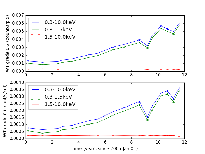
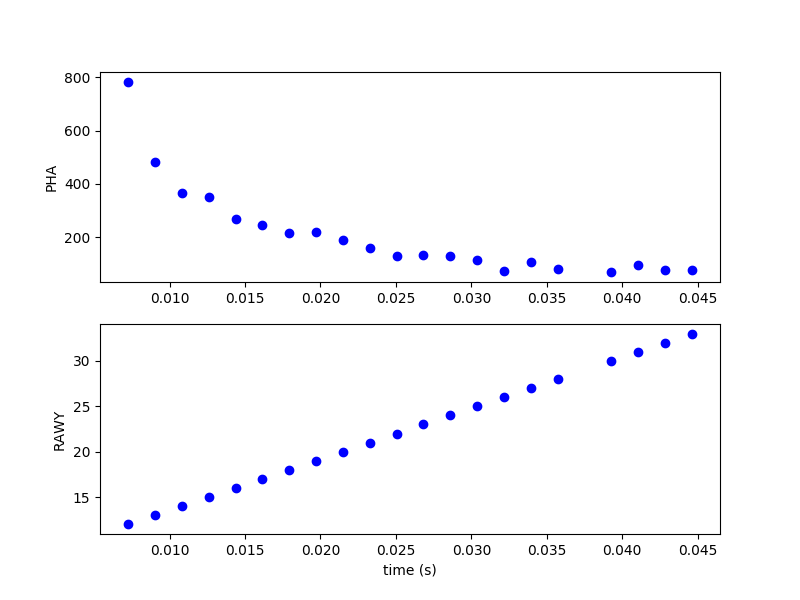
Figure 5 (left) This shows how the background levels in WT mode (Top: grades 0-2; bottom: grade 0) over the total (0.3-10 keV; blue), soft (0.3-1.5 keV; green) and hard (1.5-10 keV; red) energy ranges change. An increase in the background level with time can be seen.
Figure 6 (middle) Comparison of a WT spectrum without (black) and with (red) removal of the excess trailing charge.
Figure 7 (right) This shows the release of trailing charge from a deep trap in column DETX=349, which appears as energy dependent decay in that column in consecutive WT time bins. The top panel shows the measured PHA values (approximately 2.7 eV/DN), while the bottom panel shows that the trailing events appear in consecutive readout rows (RAWY). The time axis is plotted in seconds; WT readout time is 1.78 ms.

A method to identify and remove the trailing charge from WT event files was implemented from HEASoft 6.26 (2019 May) onwards. Results are shown in Figure 6 above, where the red spectrum was been generated after removal of the trailing charge, thus reducing the low energy turn-up.

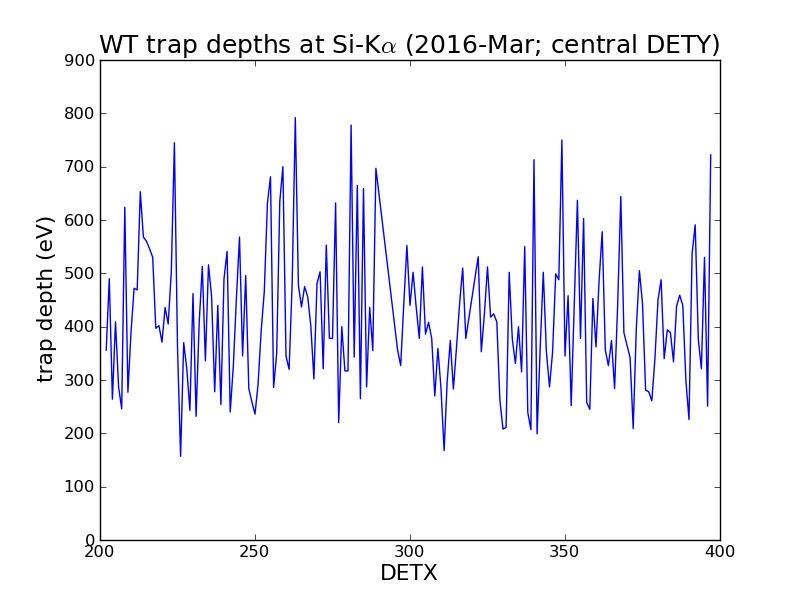
For additional reference, Figure 8 shows the depth of the traps as currently identified in the WT gain file (as of 2016 March). The deepest traps occur at DETX columns 224, 263, 281, 340, 349. Events in these columns will show the effects of trailing charge most clearly.

Figure 8 Trap depths across the central 200 pixels of the XRT CCD.

Energy Scale Accuracy

Residual energy scale offsets of ∼10−20 eV can sometimes be seen in spectra at energies near ∼0.5 and ∼2 keV, which increase to ∼30−40 eV at energies close to the iron Kα region (6.4 keV). The offsets manifest themselves as ~10% residuals around the instrumental edges (e.g. O-K 0.545 keV, Si-K 1.838 keV and Au-M 2.35 keV) in continuum sources with good statistics. Careful use of the gain fit command in xspec (allowing only the gain offset term to vary) can alleviate these residuals.

The offsets are likely caused by observations whose CCD temperatures are outside the nominal calibrated range of the gain file, or by optical loading caused by bright earth contamination.

For example, the median CCD temperature for observations during 2017 (including calibration) was −58.7 C, with 90% of the observations spanning the range -63.0 to -54.0 C; due to limited data, the energy scale is not as well calibrated for observations taken outside this range.

Occasionally, extreme CCD temperatures are reached: for example, an observation of PKS 0548-322, taken from 2018 June 03-05, was much colder than average, in which the CCD temperature ranged from -69 to -74C. This revealed energy scale offsets of ~100 eV (to higher energies) which caused the spectrum to appear heavily cut-off below ~0.5keV.

The CCDTemp value is stored in the *.mkf file (after xrtpipeline has been run) and can be examined with the FTool fv.

Low energy spectral residuals in Windowed Timing Mode

Sources which are heavily absorbed (columns of about 10²² cm^-2 and above) can show a 'bump' in the spectra at low energies (between 0.4-1 keV) and a turn up at the very low energy end. The bump is only present in event grades 1 and above (although the redistribution tail - where the data turn up - is always present). If a source is in WT mode and absorbed, we recommend extracting both grade 0 and grades 0-2 spectra and comparing them. If the bump is present, then grade 0 only should be used, since the current grade 0-2 uniform illumination RMF does not model the bump well. The presence and size of these features is a function of the source position on the detector.

Even moderately absorbed sources (few 10²¹ cm^-2) can show a turn-up in the data/model ratio plot. The energy at which this turn-up occurs is time dependent: in 2008 it is ~0.4 keV, in 2013 it is ~0.6 keV. Such features are likely not intrinsic to the source, but also due to slight RMF redistribution modelling issues, compounded by traps (see above), in this mode. Data below this energy should be excluded when fitting these absorbed sources. These issues are likely to be remediated in a future calibration release.

The position-dependent WT RMFs, released in June 2014, should help alleviate these issues. See the information page for more details about these files.

Figures 1, 2 and 3. The left-hand image shows the WT spectrum of Cyg X-3, a highly-absorbed source. The black spectrum includes grades 0-2 and clearly shows the redistribution 'bump' between 0.4-1 keV. The red spectrum (grade 0 only) does not show this 'bump', but both spectra show the turn-up at low energies. The middle and right-hand images show the moderately-absorbed Cyg X-1, again with black for grades 0-2 and red for grade 0. The middle image uses an older version of the RMF (20010101), while the right-hand image uses the epoch-dependent (20090101) RMF, which helps to model the low-energy turn up better. In the case of Cyg X-1, the 'bump' is not evident, since it is less absorbed.

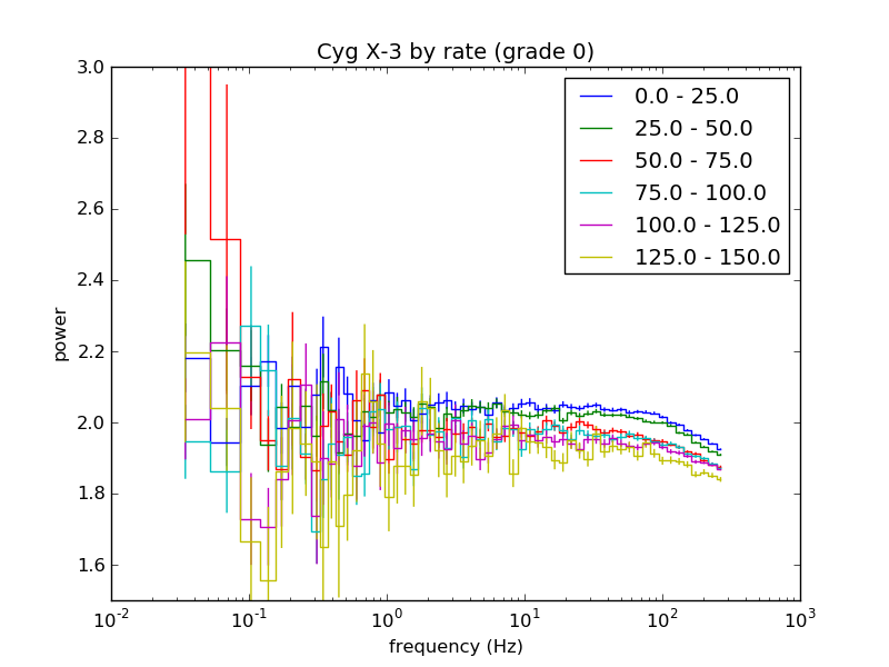
Power Spectra in WT mode

Power spectra created from light-curves extracted at the WT mode time resolution of 1.78 ms may show a drop-off at high frequencies (above about 50 Hz; see Figure 9 below), which is related to the read-out method. WT data are clocked out into the serial register 10 rows at a time. Events which would be classed as grades 1, 3 and 5-12 in PC mode and which happen to fall across this 10-row boundary will be split into 2 events of lower energy; this can affect about 2% of the events from a typical powerlaw-like source. Because WT grade zero events include some vertically split events (those classified as grades 1 and 3 in PC mode), this drop-off cannot be entirely avoided by grade selection.

Figure 9 Power spectrum of Cyg X-3, demonstrating the drop-off at frequencies above about 50 Hz.

This fall off in power has been confirmed by detailed simulations of the WT mode readout scheme. The simulations include a complete description of the charge-cloud spreading associated with X-ray interactions and resultant 10 row binning induced event splitting. As Figure 10 (below) shows, the effect is energy dependent, tracking the linear absorption depth of X-rays in the Silicon (as shallow interactions form predominantly single pixel events, while deep interactions form multi-pixel events which are susceptible to splitting at the 10 row boundaries).

Figure 10 WT power spectra simulations at various monochromatic input energies showing the energy dependence imposed on the mean noise power level caused by the WT mode readout.

In addition, if a source suffers from pile-up, the power at all frequencies is suppressed and the overall level falls below a mean value of 2 (as expected for Poisson noise when the powers are normalised following Leahy et al), as shown below.

Figure 11 This plot demonstrates how the power level changes with count rate: as the rate increases and pile-up becomes an issue, the overall level drops below a power of 2.

Baseline Subtraction

Occasionally, if a cosmic ray hits the baseline, it corrupts a line in the bias map. When baseline subtraction occurs, this row becomes apparently "hot". All the events will be rejected during the pipeline processing, so the only time when this row becomes visible is in an exposure map. An example is shown below.

Figure 12 An example of a horizontal "bad row" caused by a cosmic ray hitting the baseline.

Background features

The X-ray background detected is a combination of the Cosmic X-ray background, electronic noise and particles (cosmic rays, solar protons etc.) The WT background spectrum can be quite variable, sometimes showing a strong Nickel line at 7.5 keV and sometimes a dip between 2-3 keV. Examples are shown below.

Figures 13 and 14 The left-hand image shows a background WT spectrum with an obvious Nickel line (due to the
plating on the camera surfaces). Fig. 14 (right-hand image) demonstrates that a "lack" of counts can sometimes be
observed around 2-3 keV.

WT PSF Corrections

If part of the WT core PSF is excluded, either for pile-up or the presence of bad columns, the uncertainty of the PSF correction from xrtmkarf may be up to 10-15%.

CLOSED ISSUES

Substrate Voltage change

On 2007-08-30, the XRT CCD substrate voltage was raised from 0V to 6V as part of a plan to improve its performance at the relatively high temperatures at which it has to operate (up to -50C).

Experimental data taken with the flight spare CCD at the Leicester calibration facility had shown that by raising the substrate to 6V, the CCD dark current level would be reduced. This has been confirmed in orbit: Figure 15 below shows a measure of the thermally-induced dark current (calculated as the mean of the noise peak minus the mean of the bias level) as a function of CCD temperature, with the CCD substrate voltage at both 0V (blue circles) and 6V (red triangles). This shows the benefit of raising the substrate voltage: for the same level of dark current, the CCD can operate 3 to 4C higher with the substrate voltage at 6V compared with 0V, and thus can provide useful scientific data at hotter temperatures.

Figure 15 Comparison of the dark current at different CCD temperatures for
different substrate voltages. An increased substrate voltage allows the CCD to
operate at higher temperatures for the same level of dark current.

However, by raising the substrate voltage in this way, we expect the CCD depletion depth to decrease slightly, which will cause a small drop in Quantum Efficientcy (QE) at high energies. Observations of calibration sources before and after the substrate voltage change reveal a drop in QE of ~8% at 6 keV (Godet et al. 2007), consistent with Monte-Carlo simulations of the RMF.

Residuals around the Silicon and Gold edges

Residuals of about 10% around the Si and Au edges (around 2 keV) were previously apparent in high signal-to-noise spectra. Improved calibration files have noticeably decreased such residuals. Note that, if the energy scale is off by 10 eV or more, residuals may still be seen.

Bias-induced Energy Offsets

See this short calibration document on energy scale offsets.

Bias maps

Please note that the bias maps obtained between days 200 and 214 (19 July - 2nd August) of 2006 were incorrect. This means that there is a potential that the bias map values were too low, meaning that photon energies could appear too high - i.e., a gain offset. It also caused a temporary upsurge in hot pixels.

ARFs and RMFs

Before version 2.4 of the software (release date of 2006 April 26), there were two versions of the Ancillary Response File (ARF) which could be generated for the Photon Counting (PC) and Windowed Timing (WT) modes: empirical (the default when running xrtmkarf) and physical (obtained by typing xrtmkarf inarffile=none) files. Note that this is no longer the case for more recent versions of the software. The empirical ARFs were produced by comparing the observed Crab off-pulse spectrum (between phase 0.5 and 0.8, chosen to limit pile-up effects) with standard parameter values (Γ = 2.1; normalisation = 9.2 photon keV^-1 cm^-2 s^-1 at 1 keV) and "tweaking" the ARFs until these match as closely as possible.

There are certain differences between the ARFs which users should be aware of. In general, the physical ARFs do not model the gold edge (i.e. between 2-4 keV) very well. The empirical ARFs should not be completely trusted below about 0.6 keV.

The uncertainties at lower energies can manifest themselves as an apparent excess absorbing column of up to 10²¹ cm^-2.

Examples are shown below.

Figure 16 An example of a broad-band fit to a GRB spectrum, showing the results using both the
physical and empirical ARF files. The fit parameters were
tied together for both ARFs.

Figures 17 and 18 Close-ups of the two problem areas - the lowest energies (Fig. 17, left panel)
and around the gold edge (Fig. 18, right panel). Note that the energy axes are plotted in
linear space for clarity. Some of these residuals may be linked to energy offsets and the RMF redistribution.

Work on both the ARFs and the corresponding response matrices (RMFs) is ongoing. We caution users not to apportion high significance to observed spectral features unless a thorough investigation (using different ARFs) has been performed.

The latest documentation relating to the ARFs and RMFs can be found here.

Attitude Control

On 2007-08-11, Swift experienced an attitude control problem, which led to the observatory being offline for a number of weeks (see GCN Circ. 6760, 6797 and 6946 for more details. Because of this problem, the accuracy of Swift's slewing was poor during September and October 2007. Versions 2.8 onwards of the Swift software filter out times of particularly bad attitude. However, earlier versions of the software do not, meaning that there can be apparently multiple images of the source in sky coordinates (see Figure 19 below). Data obtained between 2007-08-11 and 2008-10-19 should be treated with caution.

Figure 19 An example of a case where the attitude was poor and the Cas A remnant was actually allocated incorrect
sky coordinates for one of the orbits. Processing the data with v2.8 of the
software filters out the time of bad attitude.