- Home
- About
- Support
- Data Access
- Data Analysis
- Data Products
- Publications
-
Links
Databases NED Simbad GCN circulars archive GRB data table Software & Tools Swift Software (HEASoft) Xanadu WebPIMMS Institutional Swift Sites GSFC PSU OAB SSDC MSSL University of Leicester
Source detection and position determination
This thread assumes that the user has already run xrtpipeline to generate the required images.
Detecting sources
In some cases, the user may wish to determine whether a source is significantly detected at given coordinates. The simplest way to do this is to use XIMAGE, which includes a sliding-cell detection algorithm. Note that, by default, the signal-to-noise threshold is set to 2-sigma. In the example below (using GRB 091029), this is changed to 3-sigma. There are also additional commands which can be included to help minimise spurious detections caused by bright sources, for example; see the discussion in Section 4.1 of Puccetti et al. (2011).
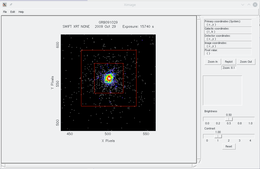
>ximage
>read sw00374210000xpcw3posk.img
>cpd /xtk
>disp
cpd /xtk displays the image in a window which allows the user to zoom-in or out (using buttons to the right of the window, or the left and right mouse buttons respectively) and re-centre (by clicking the middle mouse button).
>detect/snr=3
 Calculating background: Poisson statistics assumed
          16   1.26990257E-02
          32   8.77461676E-03
          64   8.07482097E-03
         128   6.71895361E-03
 >>> Optimum box size = 128
 Background box size = 128
 Background =6.7190E-03 cts/original-pixel
            =6.7190E-03 cts/image-pixel
            =2.7654E-04 cts/sqarcmin/s
            =4.2686E-07 cts/original-pixel/s
 Source box size (orig pix):    8 (image pix):    8
 >>>>> Searching for excesses
    791 excesses found
 >>>>> Removing contiguous sources
 Using fast contiguous search
         67 excesses left
 >>>>> Sort by radius
 >>>>> Applying thresholds
  Using average energy for PSF:    1.00000000
  snr threshold =    3.00000000
  bgnd fluctuation probability limit =    9.99999975E-05
 >>>>> removing duplicates
   #   count/s    err         pixel      Vig  RA(2000)   Dec(2000)   Err  H-Box
                             x     y     corr                        rad  (sec)
    1 1.45E-03+/-3.8E-04   505.1   525.7 1.00 04 00 41.3 -55 58 33.9  -1     18
    2 1.83E-01+/-4.1E-03   501.6   556.9 1.01 04 00 42.3 -55 57 20.2  -1     15
    3 3.43E-02+/-1.7E-03   511.4   550.6 1.01 04 00 39.5 -55 57 35.1  -1     18
    4 1.49E-03+/-3.9E-04   473.5   557.7 1.01 04 00 50.2 -55 57 18.4  -1     15
    5 4.34E-02+/-1.9E-03   491.0   557.5 1.01 04 00 45.3 -55 57 18.9  -1     18
    6 9.43E-04+/-3.1E-04   429.8   541.1 1.02 04 01 02.5 -55 57 57.5  -1     18
    7 2.21E-03+/-4.7E-04   490.7   572.4 1.02 04 00 45.4 -55 56 43.7  -1     15
    8 1.12E-03+/-3.4E-04   504.8   585.4 1.02 04 00 41.4 -55 56 13.2  -1     15
    9 1.38E-03+/-3.7E-04   371.7   537.0 1.06 04 01 18.8 -55 58 06.9  -1     20
   10 2.27E-03+/-4.8E-04   628.1   559.7 1.06 04 00 06.8 -55 57 13.3  -1     15
   11 9.67E-04+/-3.2E-04   574.8   620.5 1.06 04 00 21.8 -55 54 50.4  -1     20
   12 1.58E-03+/-3.9E-04   413.3   377.7 1.07 04 01 07.1 -56 04 22.5  -1     20
   13 1.07E-03+/-3.3E-04   615.7   601.6 1.08 04 00 10.3 -55 55 34.7  -1     18
   14 1.02E-03+/-3.3E-04   296.9   530.6 1.14 04 01 39.8 -55 58 21.5  -1     18
   15 1.81E-03+/-4.5E-04   586.4   227.3 1.32 04 00 18.4 -56 10 17.1  -1     20
   16 3.86E-03+/-6.4E-04   727.0   676.9 1.33 03 59 39.1 -55 52 36.3  -1     25
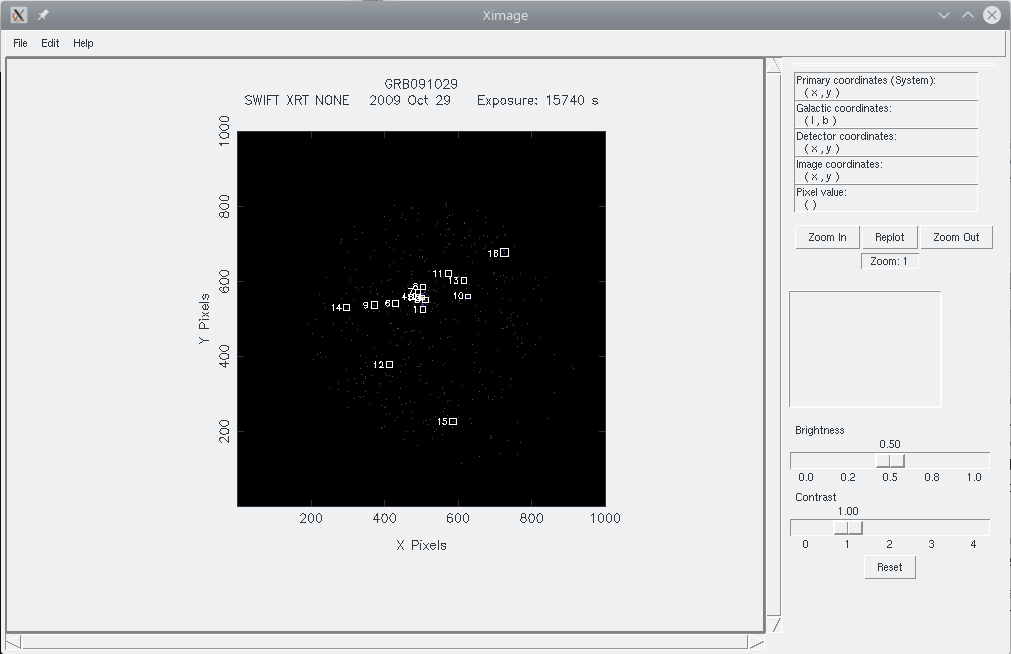
All the detected sources will be marked with a number on the image as above. If one of the source is particularly bright, the detection algorithm may pick up additional "sources" in the wings of the PSF, as shown below in the zoomed-in version:
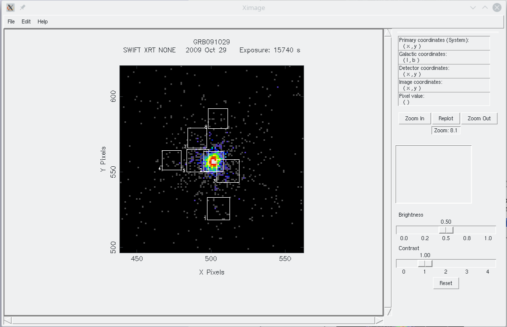
This can be circumvented by using the command detect/bright/snr=3, which merges the very nearby "detections". Note, however, that if there is a real nearby source, it will not be picked up. The output from running detect/bright/snr=3 is shown here:
Puccetti et al. (2011) used a further optimised command:
detect/bright/back_box_size=32/prob_limit=4e-4/snr=2.5/source_box_size=4.
The XIMAGE/detect algorithm is not infallible: sometimes a source will appear to be detected by eye, yet detect will not pick it up. In this case, the use of XIMAGE/sosta is recommended. sosta does not, however, determine a position of the source, whereas detect does.
sosta
Sosta ('source statistics') uses a local background to determine the significance of a source and its count rate, rather than the global background estimate used by detect, so is typically more accurate. The user is prompted to select the position of the source, at which point the background, source counts, count rate and significance of the detection are calculated. Continuing from the previous example (so the image has already been read into XIMAGE and displayed - typing disp again will clear any source detection boxes if you wish to remove them, along with zoom/repositioning commands), then:
>sosta
 Using MAP1
 Using a locally computed background
 Select the center of source box (Right button exits)
                    X = 501.17502    Y = 557.18445
  Using average energy for PSF:    1.00000000
 Source half-box for 0.65 EEF is    5.2 pixels
        Half-box for 0.90 EEF is   18.1 pixels
 Total # of counts 1800.0000 (in 121 elemental sq pixels)
 Background inner radius:   19.0 pixels; outer radius:   36.2 pixels
 Innerbox counts 2439.0000 in 1444 sq or pixels
 Outerbox counts 2650.0000 in 5184 sq or pixels
 Background counts 211.00000 in 3740 sq pixels
 Background/elemental sq pixel :                5.642E-02 +/- 3.9E-03
 Background/elemental sq pixel/sec :            3.584E-06 +/- 2.5E-07

 Source counts :                                1.793E+03 +/- 4.2E+01
 s.c. corrected for PSF :                       3.108E+03 +/- 7.4E+01
 s.c. corrected for PSF + sampling dead time
                                + vignetting    3.139E+03 +/- 7.4E+01
 Source intensity :                             1.139E-01 +/- 2.7E-03 c/sec
 s.i. corrected for PSF                         1.974E-01 +/- 4.7E-03 c/sec
 s.i. corrected for PSF + sampling dead time
                                + vignetting -> 1.994E-01 +/- 4.7E-03 c/sec <-
 Signal to Noise Ratio             :            4.226E+01


    Exposure time                 :      15740.324 s
    Vignetting correction         :      1.010
    Sampling dead time correction :      1.000
    PSF correction                :      1.733
    Optimum half box size is      : 20.500000 orig pixels
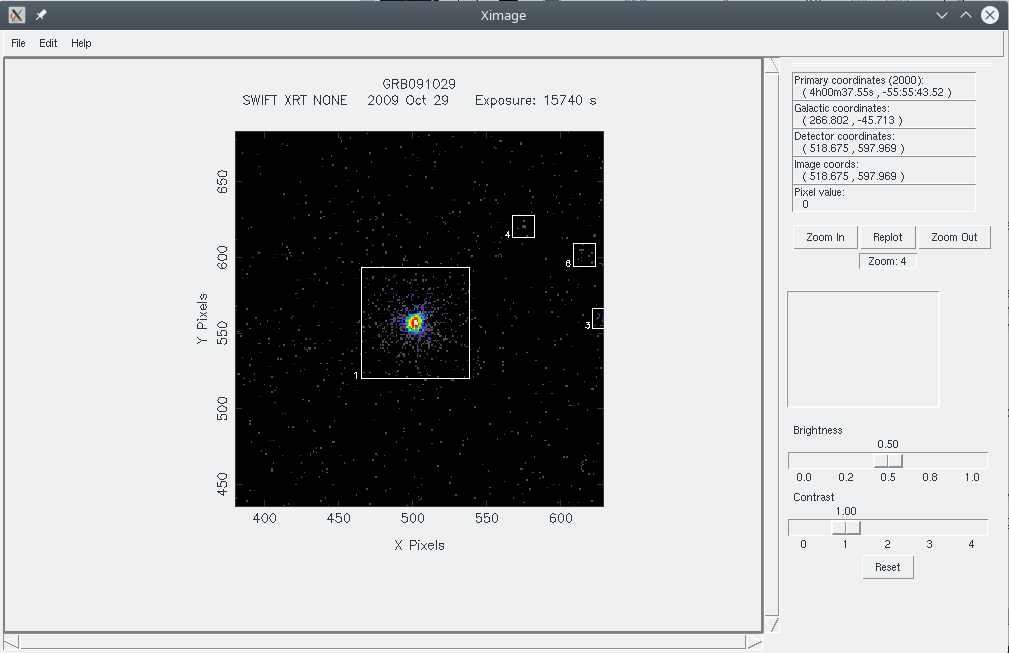
The red box-annulus shows the region from which the background rate was determined.
The detection significance is given by the "Signal to Noise Ratio" line which, in this case, is 42.26. (For a source so obviously detected, sosta is not really required!) Note that the number of counts and intensity are not corrected for any loss of counts caused by the source position overlapping bad columns. This correction factor (see the exposure map and ARF threads for details on how to calculate this value) needs to be applied separately to determining the correct count rate.
Alternatively, the online XRT product generator at https://www.swift.ac.uk/user_objects also provides a source detection option. This is based on the algorithm described by Evans et al. (2020).
Position determination
Below we explain how to determine the position of a source in the XRT field of view, using the Swift FTools. Alternatively, the best XRT positions for GRBs are available on the Enhanced Swift-XRT positions page. Note that these positions are determined using the UVOT for an astrometric correction, so will not be perfectly centred on the apparent position of the XRT source. The online tool for building Swift-XRT products allows the user to determine an astrometrically-corrected position (where possible) for any object; where this positional enhancement fails, an improved "PSF-fitted" position will be provided.
If the user does not know the coordinates of their source of
interest, xrtcentroid is one method to determine a
position. The script calls the centroiding task in XIMAGE (the same function as detect calls), but
also calculates the uncertainty on the position (by accessing the CALDB). Either an eventlist or a sky
image can be used as an input to xrtcentroid. The output uncertainty is a combination of the systematic and statistical errors, summed in quadrature (at the 90% confidence level).
Note that the systematic error for XRT positions calculated in this way is 3.5 arcsec, so will almost always dominate the uncertainty.
This position is based on the star tracker attitude solution and can usually be improved by using the UVOT for astrometric correction (see the online XRT products tool).
Using GRB 091029 as an example:
>xrtcentroid

           Running xrtcentroid version 0.2.7

Name of the output file or DEFAULT to use standard name [ ]: position.txt
Name of the output directory [ ]: ./
Calculate centroid position (yes/no)? [ ]: yes
Name of the input Event/Image FITS file [ ]:
sw00374210000xpcw3posk.img
Use cursor to define center and size of box (yes/no)? [ ]: yes
xrtcentroid_0.2.7: Info: Output Directory: './'
xrtcentroid_0.2.7: Info: ./sw00374210000xpcw3posk.tcl successfully written
 No of detectors read in:   25
 Telescope SWIFT XRT
 Image size = 1000 x 1000 pixels
 Image rebin = 1.
 Image center = 500.5, 500.5
 Using gti for exposure 2964.29462 s
 Reading an events file
 File contains      31714 events
 Accepted: 31714 Rejected: 0
  Image level, min = 0.0000000 max = 97.000000
 Copied MAP1 to MAP9
 Plotting image
  Min =  0. Max =   97.
 Using MAP1

 Select center of box
 Cursor is active
An image will then pop up, as when running XIMAGE (see above).
The user should zoom into the burst (to do this, click on the zoom in
button on the right-hand panel; unfortunately, you cannot centre the source, since
clicking within the field of view starts the centroiding process),
and click first as close to the centre of the target as possible and then just
at the edge of the source, where the PSF fades into the background. A calculated
position will then be written both to the
screen and the output file (position.txt in this example):

 Calculated centroid:

   RA/Dec (2000) = 04 00 42.2604   -55 57 18.2172
   RA/Dec (2000) = 60.1760849778   -55.9550603321

   LII/BII = 266.83 -45.69
   X/Ypix = 501.88080 557.79865

xrtcentroid_0.2.9: Info: processing '/usr/local/swift//caldb34/data/swift/xrt/bcf/instrument/swxposerr20010101v003.fits' CALDB file
xrtcentroid_0.2.9: Info: Error radius (arcsec) = 3.53920750335502
xrtcentroid_0.2.9: Info: .//position.txt successfully written