- Home
- About
- Support
- Data Access
- Data Analysis
- Data Products
- Publications
-
Links
Databases NED Simbad GCN circulars archive GRB data table Software & Tools Swift Software (HEASoft) Xanadu WebPIMMS Institutional Swift Sites GSFC PSU OAB SSDC MSSL University of Leicester
1SXPS Catalogue Creation
Search catalogue | Documentation | Refereed paper | Table descriptions | Download catalogue files | Upper limit server.
This catalogue has now been superseded by 2SXPS.
Contents
Other documentation:
1. Introduction
This web page describes how the 1SXPS catalogue was created. This information is also available in full detail in the refereed catalogue paper. This web page, although containing much overlap with the paper, is not intended to contain as much detail as the paper.
The Swift X-ray telescope has a 12.3′ radius field of view, a 0.3—10 keV bandpass a peak effective area of 110 cm2 at 1.5 keV; a PSF with HEW=18′′ and a spectral resolution of ~140 eV at 6 keV. This level of sensitivity, combined with Swift's unique observing strategy (described below) gives it a unique insight into the population of X-ray sources; particularly those which are variable or transient in nature. Swift is in a low-Earth orbit, limiting individual exposures (called ‘snapshots’) to ≤2700 s in length (the mean snapshot is ~750 s long), but its rapid slewing capability allows it to immediately slew to observing a new object as the previous target goes into eclipse, meaning Swift is actively collecting XRT data ~75% of the time. The majority of the remaining time is taken by passage of the satellite through the SAA. If the observing time requested is longer than can be satisfied in a single snapshot, a second (and third, fourth etc.) snapshot will be taken on future spacecraft orbits. The Swift observing schedule is organised daily, and ordinarily the data from all snapshots for a given source taken on the same day are stored in the same file; this collection is referred to as an ‘observation’ (which may comprise multiple snapshots), uniquely identified by an obsID. Sources observed on more than one day will thus have multiple observations in the archive.
Swift's primary goal is the detection and follow-up of Gamma Ray Bursts (GRBs), but it is also frequently used for Target Of Opportunity observations, of which many are monitoring campaigns (similar to GRB follow up). This means that Swift observes many fields on the sky multiple times over periods from days to months or even years; it is therefore an excellent tool for probing X-ray variability on multiple timescales.
As GRBs are distributed homogeneously on the sky, Swift's sky coverage is largely uniform, with a few well observed regions (e.g. the Galactic plane; see Fig. 1). This catalogue contains all Photon Counting mode XRT data observed up to 2012 October 12, which covers 1905 square degrees (nearly 5% of the sky) with at least 100 s of exposure.
Two previous XRT point-source catalogues have been produced, which used the routines built into
the ximage software to detect sources. The first, SwiftFT (Puccetti
et al 2011), analysed the deepest GRB fields, combining all of the data into a single image per field.
The second, 1SWXRT (d'Elia et al. 2013), analysed 7 years of XRT
data, considering each observation independently. For this catalogue we have developed a new detection method
capable of detecting fainter sources than these papers, and have conducted a rigorous analysis of our completeness
and false positive rate; we have also considered both individual observations and deep images,
making this a more complete point source catalogue than the 1SWXRT and SwiftFT catalogues.
| Name | Energy range |
|---|---|
| Total (band0) | 0.3—10 keV |
| Soft (band1) | 0.3—1 keV |
| Medium (band2) | 1—2 keV |
| Hard (band3) | 2—10 keV |
| HR1 | (M-S)/(M+S) |
| HR2 | (H-M)/(H+M) |
Table 1. The energy bands and hardness ratios used in the 1SXPS catalogue.
Our analysis is conducted independently in four energy bands (Table 1).
For each detected source we produce a position and error, a
count rate in each band, two hardness ratios (Table 1), flux and spectral information, and
variability information. For all sources we also provide light curves, binned
both with a data-point per snapshot and per observation.
For sources comprising at least 50 photons in the 0.3—10 keV
band (after background photons are discounted) we also provide spectra.
These products are available for download; the spectra are ready for use in xspec.
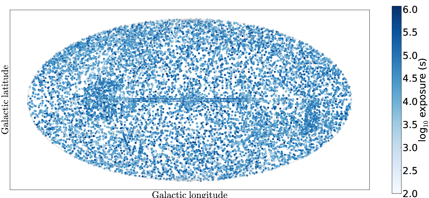
Fig. 1. Aitoff-projection map in Galactic co-ordinates of the fields included in the 1SXPS catalogue. Points (sizes not to scale) show the location and exposure of each field.
1.1 Timescales and terminology
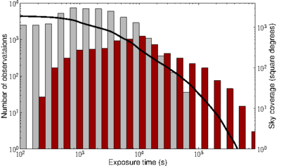
Fig. 2. The temporal and geometric coverage of the 1SXPS catalogue. The histograms show the distribution of exposure times of the observations (in grey) and stacked images (red), while the solid black line shows the unique sky coverage of the catalogue as a function of exposure time.
Swift data are organized into snapshots and observations.
Due to its low Earth orbit (P=96 min),
Swift cannot observe an object continuously for more than 2.7 ks,
thus most observations are spread over multiple spacecraft orbits.
A single, continuous on-target exposure is referred to as a snapshot.
Within a UT day (i.e. from 00:00:00 to 23:59:59 UT) the data from all
snapshots pointed at a given source are aggregated into a single dataset,
referred to as an observation and is assigned a unique
ObsID under which the data can be accessed. This is
explained further here.
In order to probe
source variability we consider both of these timescales. Neither snapshots
nor observations have a standard duration: snapshots may be 300—2700 s in duration
and there are typically 1—15 snapshots in an observation. However snapshot-to-snapshot variability probes
timescales <1 day, while observation to observation variability probes timescales >1 day.
Snapshots are generally too short for any but the brightest sources to be detected, therefore we search for sources in each observation and on summed images comprising all XRT observations on each location of the sky. We refer to these latter as stacked images. The word image where it appears in this documentation means literally as a single (FITS) image, which may be of a snapshot, observation or a stacked image; whereas field refers to an area on the sky. The term dataset refers to either an observation or a stacked image. Fig. 2 shows the distribution of exposure times in the two types of image on which we perform source detection, and the sky coverage of the catalogue as a function of exposure time.
| RA (J2000) | Dec | Source |
|---|---|---|
| 6.334° | 64.136° | Tycho SNR |
| 16.006° | -72.032° | SNR B0102-72.3 |
| 28.197° | 36.153° | RSCG15 |
| 44.737° | 13.582° | ACO 401 |
| 49.951° | 41.512° | NGC 1275 |
| 81.510° | 42.942° | Swift J0525.8+4256 |
| 83.633° | 22.014° | Crab Nebula |
| 83.867° | -69.270° | SN 1987A |
| 85.052° | -69.331° | PSR 0540-69 |
| 94.277° | 22.535° | OFGL J0617.4+2234 |
| 116.882° | -19.303° | PKS 0745-191 |
| 125.851° | -42.781° | Pup A |
| 139.527° | -12.100° | Hydra A |
| 161.017° | -59.746° | Carina Nebula |
| 177.801° | -62.626° | ESO 130-SNR001 |
| 187.709° | 12.387° | M87 |
| 194.939° | 27.943° | Coma Cluster |
| 207.218° | 26.590° | Abell 1795 |
| 227.734° | 5.744° | Abell 2029 |
| 229.184° | 7.020° | Abell 2052 |
| 234.798° | -62.467° | Swift J1539.2-6227 |
| 239.429° | 35.507° | Abell 2141 |
| 244.405° | -51.041° | SNR G332.4-00.4 |
| 258.116° | -23.367° | Ophiuchi Cluster |
| 266.414° | -29.012° | Galactic Centre |
| 299.868° | 40.734° | 3C405.0 |
| 326.170° | 38.321° | Cyg X-2 |
| 345.285° | 58.877° | 1E2259+586 |
| 350.850° | 58.815° | Cas A |
Table 2.The locations of structured or diffuse emission which can deceive our source detection. Observations with 12.5′ of these positions are excluded from the catalogue.
2. Data Selection
Our initial sample comprised XRT science observation§ carried out before 2012 October 12 that contains at least 100 s of usable exposure in Photon Counting (PC) mode. Data in other modes was not included as they do not contain the position information needed for source detection & localisation. We subsequently excluded from this sample fields overlapping the regions listed in Table 2, as those fields are dominated by large-scale structure or diffuse emission which are not handled by our background modelling and produce large numbers of spurious detections.
Our definition of ‘Usable’ data is, ‘Times unaffected by light reflected off the bright Earth, and where the spacecraft astrometry is reliable.’ We identified times of unusable data thus:
- Bright Earth
- This refers to times where the background is high due to illumination of the detector by solar light scattered off the Earth. To identify such times we examined the region on the CCD most affected by this phenomenon, which we approximated using a box 122×350 pixels centred on (62,300) in detector coordinates. Any times where the count rate in this box in the unfiltered event list exceeded 40 count/s were deemed to be affected by bright Earth contamination, and were removed from the data. For 90% of observations less than 10% of the exposure was lost to this filtering.
- Unreliable astrometry
- The spacecraft pointing is accurate to 3.5′′ 90% of the time. We identified and excluded times where the astrometry was incorrect by more than 10′′ We did this using the UV/Optical telescope (UVOT) on Swift. For each UVOT image we corrected the astrometry by matching UVOT sources to the USNO-B1 catalogue (see Goad et al. 2007 and Evans et al. 2009). We then determined the magnitude of this correction on the X-rays sources in the image and at four locations positioned symmetrically in the field at radii of 5.9′ from the field centre (i.e. mid-way to the edge of the field). If any of those were >10′′ we marked the times of that UVOT image as bad and excluded XRT data taken during those times from the analysis. It will be noted that this was a two-pass process, since it makes use of the XRT source list for a given observation, which has not been produced at this point in proceedings. We therefore ran the detect procedure in full without this phase, and then ran this astrometric checking. Any dataset containing times of bad astrometry was then re-analysed from scratch, with those times of bad astrometry removed.
§ An ‘observation’ is defined
on the observation definitions page
and refers to all data under a single obsID. By ‘science’ science observation
we mean everything except for calibration observations, which have an obsID beginning with 0006.
3. Catalogue construction
The catalogue construction consists of several processes:
- Data preparation.
- Source detection.
- Source quality flagging.
- Merging the detections across bands.
- Astrometric correction.
- Building the source list.
- Creation of the source products.
3.1 Data Preparation
All of the Swift data used in this catalogue were reprocessed locally at the UKSSDC in Leicester, using HEASoft version 6.12 and the XRT CALDB version 20120209, prior to analysis.
For the per-observation images there was only one PC mode event list per
observation† whereas the
stacked images contain multiple event lists. Our source detection software
worked in the “SKY” (X,Y) coordinate system, which is a
virtual system constructed using a tangent plane projection, such that
(X,Y) has a linear mapping to (RA,Dec) (see
Greisen & Calabretta 2002;
Calabretta & Greisen 2002).
These co-ordinates are constructed by
the coordinator FTOOL when the Swift pipeline processing is
performed, and the relationship between (X,Y) and
(RA,Dec) is different for each observation. During the construction of stacked
images we therefore called coordinator for each obsID in the image, instructing
it to use the same projection for each image, thus creating a common (X,Y) system
to use. For stacked images of GRB fields we also excluded the
first snapshot (i.e. of PC-mode data), as the image in these snapshots is often
dominated by the GRB.
From this point on the procedure for the stacked images and the single-observation images was the same and we use the generic term ‘dataset’ to refer to either an observation or stacked image. Before source detection, various steps were taken to prepare the data.
For each snapshot of data, Swift slews afresh to the target (having been observing other things in the meantime), as a result of which each snapshot has a slightly different centre and spacecraft roll angle. It was therefore necessary to split the data into snapshots, to avoid spurious features in the background maps (described later) at the edge of the per-snapshot fields of view. For each snapshot an exposure map was created (which included the effects of vignetting assuming an event energy of 1.5 keV) and an image is constructed of the grade 0—12 events in each of the four energy bands given in Table 1. The centre of the image (in SKY coordinates) and the spacecraft roll angle for that snapshot were recorded to be used by the background-mapping software. The XRT has 3 different window sizes that have been used at different times: 480×480 pixels, 500×500 pixels, and 600×600 pixels (referred to as w4, w2 and w3 respectively) and which of these was used was also recorded. Finally, the per-snapshot exposure maps were summed to give a single, total exposure map (as well as the individual files) and likewise for each band's images. These files were then passed to the source detection software.
At the end of the data preparation phase the following products had been created:
- Exposure map per snapshot
- Total exposure map
- Image per band per snapshot
- Total image per band
- File detailing, for each snapshot, the exposure map file, per-band image files, image centre, size and roll angle
†Prior to 2008 June 3 any observation spanning 00:00 UT had a second, short (<90 s) observation; these observations were not included in our analysis.
[Back to top | Back to Data Processing | 1SXPS index]
3.2 Source Detection
Source detection was performed independently for each energy band. We used a form of sliding-cell detection combined with a PSF fit to identify and localise sources. This approach was based on that employed for the 2XMM catalogue, but modified to suit our specific needs. The process contains the following elements:
- Sliding-cell detection with a locally estimated background.
- Creation of a background map.
- Sliding cell-detection using the background map.
- PSF fitting (i.e. localising a source by fitting the instrumental PSF to the image).
- Likelihood tests.
each of which is described below. The detection process is iterative, and can be summarised thus:
- Perform a high threshold (SNR=10) sliding-cell detection, using a locally estimated background.
- Create a background map, then discard the source list from the previous step.
- Perform a high threshold sliding-cell detection, measuring the background level from the map.
- If sources were detected in the previous step, then localise the brightest one using a PSF fit, and perform a likelihood test.
- Repeat steps 2—4 until no sources are found.
- Create a background map.
- Perform a normal threshold (SNR=1.6) sliding-cell detection, measuring the background level from the map.
- Localise all new sources found in the previous step by PSF fitting.
- Repeat steps 6—8 until no sources are found.
- Create a new background map.
- Redo the PSF fit on every source. Also calculate parameter errors and perform likelihood tests.
3.2.1 Initial sliding-cell detection with a local background estimate
In this first pass we looked only for bright sources. This was done using a sliding cell search, with the background estimated from an annular box around the main cell. We largely followed the process detailed in the Chandra Detect Reference Manual. We initially used a cell of 21×21 pixels (=49.5′′, this region encloses 81% of the XRT PSF), and measured the number of counts C in this cell and the Gehrels (1986) error σC=1.0+√(C+0.75). We also measured the counts in a 51×51 pixel cell with the same central location to estimate the background and uncertainty. Given the known shape of the Swift PSF, we then calculated from these numbers the expected number of photons, S, from a source in the centre of the cell, and its uncertainty σS. We used the exposure map during this calculation to correct for variations in exposure between the inner and outer cells. This, for example, prevents an artificial increase in the significance of sources at the edge of the detector. The signal-to-noise ratio of the possible source is given by SNR = S/σS.
The cell was stepped over the entire image in 7-pixel steps. Although we are looking for bright (SNR>10) sources at this time, the 21 pixel box may not be optimal. The ideal cell size is a function of the source intensity. We therefore searched for any 21×21 pixel cell with an SNR of at least 1. Such cells where then further investigated by reducing the cell size to 17×17 pixels (the background region was reduced in proportion) and stepping it around inside the original 21×21 cell. If one of these smaller cells had an SNR larger than in the 21×21 cell, then its position and size were noted. The cell was then reduced to 15×15 pixels and stepped around inside the 21×21 parent cell as before. This continued for cells of size 11, 9 and 7 pixels, until no excess with an SNR greater than in the large cell was found. Then all of the cells which were noted during this process were compared. If any cells overlapped, only the cell with the highest SNR was kept. For each cell thus found, a barycentre was calculated (using only counts within that cell), and then the box size with the maximal SNR was found. If the SNR of this cell was above the target threshold, 10 in this initial search, the cell was saved as a potential source, otherwise it was discarded. These above-threshold potential sources are referred to as ‘excesses’.
Once the entire image had been covered by the celldetect, any duplicates (i.e. excesses with identical positions and cell sizes) were reduced to a single excess, and then all excessed were sorted in increasing order of box size. Overlapping, non-identical excesses were combined, with the mean position and box size determined, weighted by the number of photons in the excess. A barycentric position within this mean box was then determined, and the box size which maximised the SNR at this position was saved. Finally, these barycentric positions were again checked for overlaps; if any were found only the excess with the greater SNR is kept. This resulted in a list of newly-detected excesses, which was the final product of the cell detect phase.
The complexity and iterative nature of this process is necessary to achieve good sensitivity to both bright and faint sources, minimise the false positive rate, and disentangle nearby sources. The efficacy of this is demonstrated in Section 5.
3.2.2 Creation of a background map
In order to achieve the optimal sensitivity and most accurate reconstruction of source parameters, it was necessary to accurately measure the background across the detector. The exposure varies across the field of view due to vignetting, and there may be genuine astrophysical variation in the background X-ray flux. To model these effects, we therefore created background maps.
The creation of the background map was repeated at almost every stage of the detection process. It had to be performed for each snapshot individually (since the snapshots each have unique centres and roll angles), and the per-snapshot maps were then combined into a single map. The procedure detailed below is that conducted per snapshot. Fig. 3 shows an example of the main steps.
First a detector mask was created. Pixels in the detector map can have a value of either 1 or 0; by default all pixels were set to 1 (even those outside the field of view). Then the mask was set to 0 in the region of every excess identified so far. With the exception of the first and last maps created, the list of such excesses comprised a mixture of excesses returned by the most recent cell detect run and all excesses which have been PSF-fitted so far. For the former, the details of the count rate and shape are not well known, so the masking was approximate: the count rate was estimated based on the box-size and the known instrumental point-spread function (PSF); and the radius at which the count rate dropped below 10-5 ct/sec/pixel is determined; pixels out to this radius were masked, to a maximum radius of 150 pixels. For PSF-fitted excesses, where the PSF profile and count rate were better known, the mask radius was that where the count rate dropped to 10-6 ct/sec/pixel (a typical background level for an XRT exposure), again with a maximum of 150 pixels. If this process resulted in more than 80% of the image being masked out, the mask radius was reduced by 5% and the process is re-performed.
The mask was net multiplied by the image for the current snapshot to
create a masked image (called a Swiss-Cheese image in the XMM and
Rosat papers; Watson et al
2009; Voges et al. 1999).
This image was then divided by the exposure map (pixels with 0 exposure were given a value of 0) and
rebinned into a 3×3 grid. This grid was centred on the image centre,
rotated to match the spacecraft roll angle, and set to the size of the image (as defined in Data Preparation, above); there could be no photons outside this
region. The mean background level in each of the 9 cells thus created was determined by summing
the values of demasked_image/exposure_map for each unmasked pixel in the bin for which the exposure map had a non-zero value
and then dividing by the number of pixel included. The uncertainty in each of these cells was calculated
using the Gehrels (1986)
approximation that, for a cell with C photons, σC=1+√(C+0.75).
If a cell contained no unmasked events then its value and uncertainty were set
by interpolation (or extrapolation if necessary) from the neighbouring cells. The background map
was then created by treating the central pixel of each cell as having the value of that cell and
then using bilinear interpolation to determine the background map value in each image pixel with non-zero exposure, and
multiplying by the exposure map to get a map of the background intensity.
The uncertainty in each pixel was also propagated through
these calculations, giving a background error map.
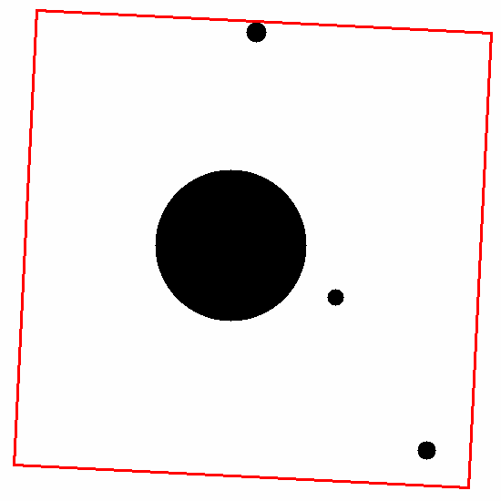
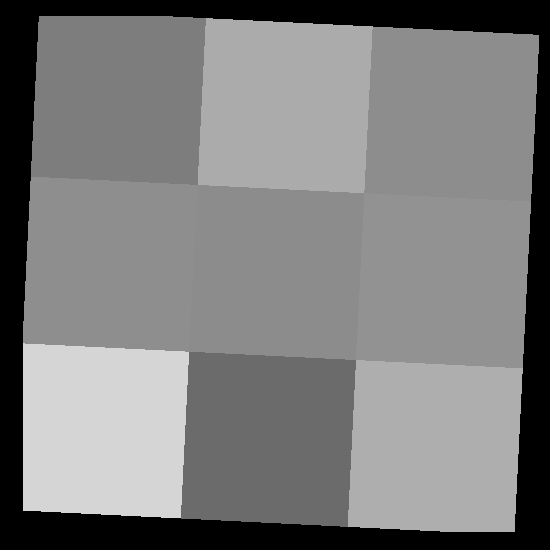
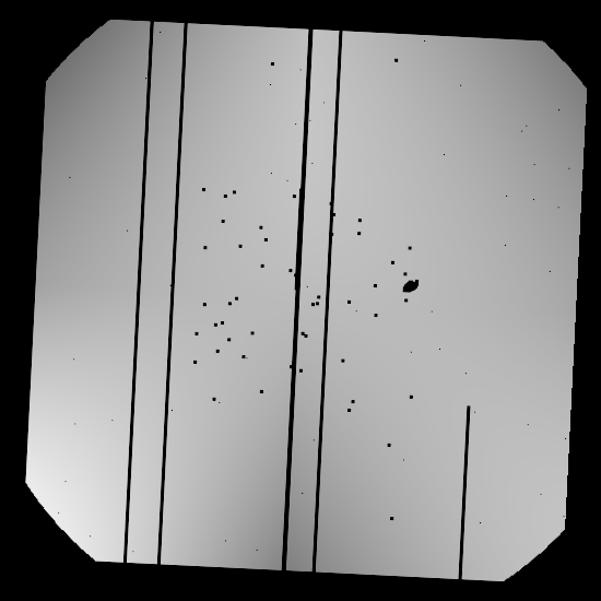
Figure 3 An example of the background map creation process.
Left: The detector map, with four sources detected in earlier iterations masked out.
Centre: The rebinned background.
Right: The resultant background map after interpolation from the previous step, and dividing by the exposure map
Finally, any sources which had been localised (and characterised) by PSF fitting were added back into the background map, by adding the model PSF to the map. The azimuthal variation caused by the shadow of the mirror support structure was included in the PSF model used. This both makes it easier to detect sources which are close together, and reduces the number of spurious detections in the wings of brighter sources. For sources brighter than 3 ct/sec, out of time events (photons which strike the CCD while it is being read out) become comparable to the background level of a typical observation, and were also added to the map. Fig. 4 shows the resultant background map after all of these steps have been taken.
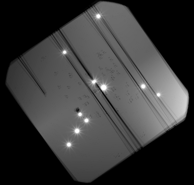
Fig. 4 A completed background map, after all snapshots have been combined and the detected sources included.
We confirmed that our background mapping was working properly using simulations, as discussed in Section 6.
3.2.3 Sliding-cell detection using the background map
After the first background map had been created, each new detect pass followed the sliding cell method as described earlier, with one difference: instead of estimating the background level from an annular box, the background level and its error were taken from the background map at the location of the current cell. Thus the number of source photons in the cell was given simply by S=C-B where C and B are the counts in the image and background map respectively, within the test cell. Similarly the uncertainty σS=√(σC2 + σB2). In the first instance the SNR threshold required for detection was 10, and only the highest SNR excess was saved. This is because spurious detections are common in the vicinity of bright objects, so by accepting only the brightest excess at each step (i.e. the one most likely to be the actual source) and then inserting this this excess into the background map, the likelihood of finding a spurious excess around this object was reduced. Only when no more bright sources have been found was the SNR reduced to its normal level of 1.6. At this point the initial cell size was reduced from 21×21 pixels to 15×15. This is because lower SNR sources are fainter, and thus their PSF wings disappear at smaller radii; by reducing the initial cell size nearby sources can be more easily disentangled. Once a potential excess was found in this 15×15 cell, the process of searching smaller sub-cells was performed, as in the initial detection.
3.2.4 PSF Fitting
| SNR | PSF Fit radius |
|---|---|
| ≤7 | 12 pixels |
| 7< SNR ≤ 11 | 15 pixels |
| 11< SNR ≤ 40 | 20 pixels |
| SNR > 40 | 30 pixels |
Table 3. Radius of the circular region used for PSF fitting as a function of source SNR. 1 pixel=2.357′′
At each iteration, the newly detected sources were localised accurately using a PSF fit which minimised the Cash C-statistic. This took the image, exposure map and background map in a circular region centred on the position returned by the cell-detect routine. The size of this region depended on the SNR of the source, as tabulated in Table 3. We fitted a series of PSFs, starting with that in the CALDB and then a set of profiles to represent increasingly piled-up sources, as developed by Evans et al (2009). Based on simulations, we required that the C-statistic had to improve by at least 10 before accepting a fit as being better than a fit using a less-piled-up PSF. The count rate of the source was then determined from this fit, and corrected for pileup and other instrumental effects (bad columns, vignetting etc., via the exposure map) as follows. A region was defined with the outer radius set according to Table 3 and the inner radius set from Table 4. The number of photons in the image and background map within this region were recorded, as C and B respectively. If C-B>30 the number of source counts was taken as S=C-B ± √(C+B), otherwise it was determined using the Bayesian method of Kraft, Burrows & Nousek (1991); with the 1-σ (i.e. 68.3%) confidence interval also calculated.
Then the fitted PSF was calculated at each pixel in the region just determined, and multiplied by the exposure map at this point. Also, the CALDB PSF was integrated out to a radius of 150 pixels and multiplied by the nominal exposure time of the image, E. The ratio of these numbers gave the ‘Correction Factor’ (CF) necessary to correct for instrumental artefacts, pileup and vignetting. The count rate was then determined by R=S*CF/E. This rate was then used to build the background map during the next iteration, as described above.
| PSF | Annular radius |
|---|---|
| CALDB | 3 pixels |
| rate=0.9 | 4 pixels |
| rate=1.4 | 6 pixels |
| rate=2.6 | 7 pixels |
| rate=4.0 | 8 pixels |
| rate=5.2 | 13 pixels |
| rate=8.6 | 20 pixels |
| rate=15 | 25 pixels |
Table 4. The radii at which pile-up was deemed to no longer be a problem for the different PSF profiles. For the CALDB profile the inner 3 pixels were only excluded if the uncorrected source count rate was above 0.6 s-1. The rate values are the raw (uncorrected) count rate of the object from which the PSF was determined.
After PSF fitting we checked for any duplicate detections of the same source. These can occur because (despite including the fitted sources in the background map) the cell-detect code sometimes misidentified the wings of a bright source as a new source. We thus checked for sources which were close to each other (where ‘close’ is defined in terms of source count rate, see Table 5); if a new source was found which was too close to an existing source, it was rejected. This means that the process was in effect ‘blind’ within some given radius about any detected source, however this artificially imposed blindness was a reflection of the fact that the false positive rate within that region was high, effectively blinding the detection process anyway.
After the source detection was complete (i.e. no new sources were found) all of the sources were refitted so that the effect of each source on its neighbours could be incorporated correctly. To achieve this we rebuilt the background map, and added all but the highest SNR source to this map. Then a PSF fit was performed to localise this brightest source. Then the background map was rebuilt again, and all sources except for the second SNR source were added in (the highest SNR source was modelled at its new location and count rate) and then the second source was localised with a PSF fit, and so on until all sources had been fitted. A final check for duplicates was also performed: where found, the highest SNR source was selected and the others discarded.
| Count rate | Merge radius |
|---|---|
| R ≤0.4 s-1 | 10 pixels |
| 0.4< R ≤ 1 | 35 pixels |
| 1< R ≤ 2 | 40 pixels |
| 2< R ≤ 8 | 47 pixels |
| R > 8 | 70 pixels |
Table 5. The radii used to identify multiple detections of the same source. If sources lay within this radius of each other, they were considered to be the same source, and the one with the greatest SNR was accepted, the other(s) were rejected. 1 pixel=2.357′′
3.2.5 Likelihood testing
During each PSF fit phase, the C-statistic was also calculated with the source normalisation set to 0; i.e. with no source present. Since ΔC is distributed as ΔΧ2 (here with 2 degrees of freedom) we could determine the probability that the improvement in C-stat when a source is present is coincidence: P=Γ(ν/2, ΔC / 2); and hence the log likelihood, L=-ln(P) where Γ is the incomplete gamma function. However, as noted by Watson et al 2009, this probability cannot be interpreted as the probability that the source is real, since one of the C-statistic measurements was determined at a boundary condition of the model: where there is no source present. Indeed, the false positive levels reported for 2XMM are 10—100 times higher than predicted by the χ2 distribution (for measured false positive levels of 0.5%—2%). We instead calibrated the relationship between L and P(false) using simulations, as described in the Verification section. Based on this, sources with L<3 were rejected as soon as L is calculated. If L≥3, the source was flagged according to how likely it is to be a false positive, as described in Quality Flagging, below.
An extra check was also performed to eliminate spurious detections caused by hot pixels, hot columns and hot rows on the detector. For this, the combined event list of all observations comprising the image was considered, and events lying within the PSF-fit region were extracted. A sources was discarded unless these events covered at least three distinct detector pixels, 3 rows, and 3 columns, otherwise the source was rejected as an artefact. Furthermore, if more than 50% of the events lay in a single pixel, or 75% in a single row or column, the source was rejected.
[Back to top | Back to Data Processing | 1SXPS index]
| Flag Name (Value) | False pos rate | Cum. False pos rate |
|---|---|---|
| Good (0) | 0.3% | 0.3% |
| Reasonable (1) | 7% | 1% |
| Poor (2) | 35% | 10% |
Table 6. The flag schema. The names are referred to in the documentation, but are stored as numbers in the database. The cumulative false positive rate refers to the false positive rate in flags up to this value. i.e. the false positive rate when considering all Good and Reasonable sources is 1%, although the false positive rate among just the Reasonable sources is 7%.
3.3 Quality Flagging
Once the source detection was complete, the location of each detection was compared to a list
of known extended sources (taken from Tundo et al., 2012), the
detection was rejected if its position lay within the extent of the extended source (since this is a point source catalogue). A search
was also performed for bright optical stars which could cause optical loading, and give
spurious detections. Such sources were not removed from the catalogue, but the
ol_warn value in the results table is non-zero for such objects (the details
of the results table are below).
The next stage was to classify the reliability of each detection; we defined 3 classifications, Good, Reasonable and Poor the false positive rates for these categories are given in Table 6. Which category a source falls into was based on the likelihood value; the calibration of the likelihood thresholds for each classification is described in Section 6.2. This flag is stored in the results table as an integer value, the ‘Detection flag’ with values 0=Good, 1=Reasonable and 2=Poor. There is also a ‘Field Flag’ which is given for each observation and stacked image. It is normally 0 (indicating no problems) however for some fields has been set to a value or 1 or 2 following the visual screening described below. This indicates that the background may have been incorrectly characterised for that field.
There was an additional category of sources, Bad, with a very high false positive rate (~80%). These sourced were removed from the catalogue, and the background map used to create light curves was built without them. These detections are stored internally however and are reported by the upper limit server, if the limit at the location of a bad detection is requested.
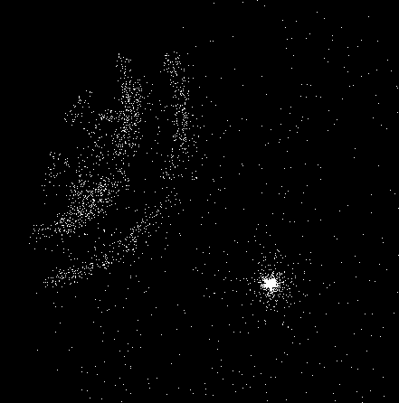
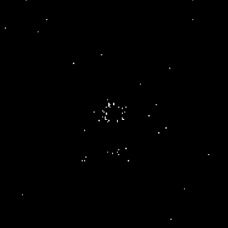
Fig. 5 Example artefacts: Left: Stray light. The concentric rings in the upper left of the image are caused by singly-reflected X-ray photons from a source 35′—75′ off axis. Right: Optical loading. The annular rings of events near the image centre is caused by a bright optical source which.
3.3.1 Visual (manual) screening
The automated quality flagging using the likelihood ratio was not able to identify spurious sources caused by astrophysical phenomena such as diffuse sources or stray light. The latter case is caused by a bright (>~3.5×10⁻¹¹ erg cm-2 s-1) X-ray source between 35′ and 75′ away from the XRT boresight, which produces concentric rings of events in the detector (Fig. 5, left). Fields lying this distance from a catalogued source were thus selected for manual inspection, additionally any field where the median distance between detections (in any band) was <80′′ were also flagged. Each of these fields was then checked by a human. If a dataset contained an ‘artefact’ that is stray light, residual bright Earth emission not completely screened out earlier, or a ‘ring of fire’ caused by a bright optical source (Fig. 5, right), the region affected was marked. Any sources lying in this region had their detection flag increased by 8 (i.e. Good/Reasonable/Poor have flag values of 8,9,10 respectively); this preserves information about the strength of the detection, while also indicating that there is a high likelihood that the source is spurious. The presence of spurious detections in an image will result in the background map being incorrect (since the model PSF for those sources is included in the map), and may introduce inaccuracies in the flux of any source in the field; the field flag for these observations or stacked images is therefore set to 2.
During the visual inspection we also checked for any regions of diffuse emission; such regions were marked as for the artefacts. Sources lying in these regions had their detection flag increased by 16, and the field flag for the image was set to 1. This field flag was also set for all fields containing an extended source in the extended source catalogue referred to above. Note that a field could only be flagged as having artefacts or diffuse emission; in the event that both effects are identified in a field, the diffuse emission settings took priority, i.e. the detection flags were increased by 16 (not by 16 and 8) and the field flag was set to 1.
Unflagged fields may still contain faint diffuse features, however these should be below the level where source parameters are significantly affected.
[Back to top | Back to Data Processing | 1SXPS index]
3.4 Merging detections across bands
The source detection procedure (described above) was performed independently on all four bands of each dataset. After this the detections had to be merged across those bands to produce a unique source list for that dataset; the sources in this list are hereafter referred to as ‘Obs Sources’. This merging was based on the radii defined in Table 5 and, where multiple detections were found, the location with the smallest error was selected as the position of the Obs Source. If multiple detections had the same error, that with the highest SNR was selected.
[Back to top | Back to Data Processing | 1SXPS index]
3.5 Astrometric corrections
The absolute astrometric uncertainty of standard Swift-XRT positions, which are based on the spacecraft attitude reported by the star trackers, is 3.5′′ (radius, 90% confidence). However it was possible in some cases to improve this. For any dataset containing more than 2 Obs Sources with detection flag <2 (i.e. Good or Reasonable and not in a region identified by visual inspection as being problematic) we retrieved a list of 2MASS objects that lie within the area covered by the dataset. We then attempted to find an aspect solution which maximised the likelihood, L=Σox<20 exp (-0.5 δ2/σ2). Where the sum is over all pairs of 2MASS/X-ray objects which are within 20′′ of each other, δ is the angular distance between the X-ray and 2MASS pair, and σ is the uncertainty in the two positions, added in quadrature. The uncertainty in the astrometric solution was determined by measuring the RMS of the δ values from each X-ray/2MASS pair in the final fit. If the mean shift in an X-ray position as a result of this process was >15′′ the solution was considered unreliable and rejected: this distance corresponds to a 7-σ inaccuracy in the star tracker solution, a most unlikely situation.
To calibration our astrometry we obtained the SDSS Quasar Catalogue (DR5) and identified all sources in our catalogue within 2′′ of these objects. We then performed the above astrometric correction for those fields, and measured the distance of the nearest X-ray source to the SDSS position from that location (provided it was within 20′′). As expected, 90% of the X-ray positions were consistent with the SDSS position at the 90% level.
This process could not find an astrometric solution for every XRT dataset: some had too few X-ray objects, for others no good solution could be found which did not require an unrealistically large solution. Also, in many cases the uncertainty on the astrometric solution was >3.5′′ in which case the Swift star tracker astrometry is better and we did not use the astrometrically “corrected” position. In total 58,725 Obs Sources in 2,437 datasets had their astrometry derived from the correlation of X-ray and 2MASS positions.
[Back to top | Back to Data Processing | 1SXPS index]
3.6 Building the source list
Once the source detection was completed for all observations, we merged the list of Obs Sources into a final catalogue of unique sources.
This was done in a manner analogous to that of the Obs Source creation (Section 3.4), except that Obs Sources were matched if their positions agreed to within 5σ**;, rather than based on their merge radius. This accounted for the astrometric uncertainty between observations, and also allowed for sources that were close to a bright source, and detected after that source had faded, to be distinguished from the bright source. The source detection flag and field flag were set to be the best (i.e. lowest) flag of all Obs Sources in that source; the optical loading information was set to be the worst value.
**Radial position errors follow a Rayleigh distribution, not a Gaussian distribution, we use the term ‘5-σ’ for familiarity, where we really mean the confidence limit including 99.9999426% of the probability, i.e. the equivalent of the 5-σ limit for a Gaussian. This is actually a radius 2.498 times the 90% error radius.
[Back to top | Back to Data Processing | 1SXPS index]
4. Catalogue products
4.1 Temporal properties
We produced light curves in each of the four energy bands, with one bin per observation and one bin per snapshot (for observations where the source is undetected the latter light curve only contains a single bin integrated over that observation). We also produced time series of the hardness ratios with one bin per observation. The times of each bin in all of these products were corrected to the solar system barycentre (i.e. TDB).
To construct the time series, the count rate in each snapshot or observation was determined as described in Section 3.2.4, except that we used the best source position determined per observation (see Section 3.4), to account for the potential differences in astrometry between observations. The source-count accumulation region used was also that from Section 3.4 if the source was detected; for bands, snapshots or observations where the source was not detected a circular region of radius 12 pixels (28.3′′) was used.
For the time series in each band we calculated used the Pearson's χ2 to determine the probability that the source was variable. This test, which reports the probability of the null hypothesis that the source is constant, was applied to both the per-snapshot and per-observation light curves in each band.
4.2 Spectral properties
To estimate the source spectrum we used multiple approaches depending on the brightness of the source, each of
which considered two standard models: an absorbed power-law and an absorbed APEC model.
For every source we derived a counts-to-flux conversion factor for a power-law with a photon index of 1.7, and
an APEC with a temperature of 1 keV. The absorption used was the Galactic value in
the direction of the source, derived from the work of Willingale et al. (2013),
and modelled in xspec with the tbabs model.
We also produced 3-D look-up tables for each of the models, of (HR1, HR2, x), producing tables for x=NH, x=photon index and x=counts-to-flux conversion for the power-law model, and x=NH, x=kT and x=counts-to-flux conversion for the APEC model. We produced two counts-to-flux conversion factors (or energy conversion factors: ECFs), for the observed flux and unabsorbed flux. For each source with an (HR1,HR2) lying in the region permitted by the power-law/APEC model, we interpolated to find the spectral properties appropriate for the HRs of the source. To estimate the uncertainty we also interpolated the spectral properties as the four HR extremes, i.e. (HR1min, HR2); (HR1max,HR2); (HR1, HR2min); (HR1, HR2max). The minimum/maximum values of the spectral parameters found in this way were interpreted as the 1-σ confidence limits on those parameters. If any of these test values lay outside the region in (HR1,HR2) space permitted by the spectral model, we took the value at the (HR1,HR2) point closest to the test values instead; if this measurement turned out to be the extreme value of a given parameter, then the appropriate error was marked as unconstrained: in the results table this is reflected by the value being +/-1, where the sign is the opposite to that expected for the error. e.g. if for a source the position (HR1max, HR2) lay outside the region covered by the lookup table, and the nearest lookup point to this contained a higher NH value than any of the other (HR1, HR2) limits, then the NH positive error is unconstrained, and set to -1 in the results table. For some sources the actual HR values are not in the area covered by the spectral model. For these cases we calculate the probability of finding the observed HRs and errors if the spectral model in question were really the correct model. This allows for the easy selection of sources whose spectra are not consistent with a simple model.
For the brightest sources, those with at least 50 net counts in
the total band image, we constructed a spectrum using the tools of
Evans et al. (2009). New XRT response matrices were released in 2013 March
and we used these matrices to fit the spectra in xspec, using both power-law and APEC
models. For these objects the results of the
spectral fit are also given in the results table. Although we performed
the fit using the C-statistic in xspec, once the best fit had been found
we calculated χ2 using Churazov weighting, and report
this in the results table.
Each of the approaches above produces four ECFs: for observed and unabsorbed fluxes assuming an absorbed power-law or APEC model. Each of these is reported, however for ease of comparing sources we also provide a field giving the “best” (or highest fidelity) observed/unabsorbed flux for each model; this comes from the spectral fit if available, if not from the 3-D lookup tables if available, and if not from the fixed models.
[Back to top | Back to Catalogue Products | 1SXPS index]
5. Catalogue verification, completeness and false positive rate
We used simulations to verify the behaviour of our analysis tools and to constrain details of the catalogue such as the false positive rate and completeness. To do this we first created a set of ‘seed’ exposures, from which simulations could be created. These were XRT observations coincident with 2XMMi DR3 fields, and therefore already well studied in X-rays. For each of these we extracted a list of 2XMM sources with fluxes sufficient to produce at least 2 photons in XRT. After visually confirming that all objects in the XRT images were included in this 2XMM list, we then passed the source list to the background mapping software described under source detection, above which created a source-free map of the background counts in the image. We did this for a range of image exposure times.
To simulate an image we then took the background map and exposure map from
a seed image, from which the number of expected background counts in each
pixel, μ, can be calculated. We then drew the actual number of background photons in
that pixel from a Poisson distribution with a mean of μ. To add sources to this image
we used the logN-logS distribution of Mateos et al (2008)
and, assuming a typical AGN spectrum (photon index of 1.7, NH=3×1020 cm-2),
drew the number of sources and their expected brightnesses at random from this distribution.
We then added each source to the image; adding C photons, where C was drawn
at random from a Poisson distribution with a mean equal to the number of expected counts
given the source brightness and image exposure time. The location of the source in the image was randomised,
and each simulated photon was folded through the instrumental PSF, and the exposure map. For the latter,
if the value of the exposure map at the location was less than the peak exposure for the image, we
define x=exposure_this_pixel/peak_exposure, and then drew a random number
between 0 and 1. If this number was ≤x, the photon was added to the image, otherwise it was not.
[Back to top | Back to verification | 1SXPS index]
5.1 Verifying the background mapping
To confirm that our background mapping was working correctly we simulated an image with no sources, using the above method. Since this image contained no sources, the true background level in the image could be measured directly from the image. We did this in by averaging the counts/pixel in a randomly-position circle of radius 60 pixels†. We then used our background mapping tool to build a map of this background, and calculated the mean value (in counts/pixel) of this map, and the average level in the same region used above. We performed 400 such simulations.
We also tested how well the background was reconstructed when a source is present, using a similar technique. We simulated an image with no sources, and measured the true background in this as above. We then added a source to this image, ran the source detection routine, and took the final background map (without sources added in) produced by this technique; reading the background level of this map as above. We performed 400 of these simulations as well.
The results of this process are shown in Fig. 6. This shows that our background mapping technique accurately reproduces the background, even when sources are present in the image.
†When the background map is used in the catalogue this region can be quite small. For the simulations we used a larger region — with a radius of 60 pixels — so as to gather a reasonable number of photons in the image, as opposed to the background map. If we used too small a region, the Poisson errors on the true background measurement are large and render the test useless.
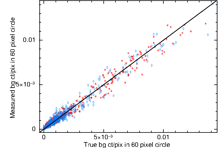
Fig. 6 The results of our simulations to test the background mapping. The x-axis shows the true background level in the simulated images in a 60-pixel circle, the y-axis shows the value from the background map in the same region. The red stars are for simulations with no sources in the image, blue diamonds are with a source in the image.
[Back to top | Back to verification | 1SXPS index]
5.2 Source detection completeness and false positive rate
As noted earlier, once the source detection was complete we manually inspected all images which lay in a location where stray light contamination was expected, or where the median inter-source distance was low. In total ~5,000 images were checked in this way. Although the main focus of this process was to identify stray light (and other instrumental artefacts) and diffuse emission, this also allowed us to verify that the detection process was behaving as expected. However, to properly calibrate the false positive rate and completeness of the catalogue we performed a large number of simulations.
Initially we simulated a series of images with discrete exposure times. A single seed image was used for each exposure. We then performed a further 30,000 simulations using a wider range of seed images. For each image the exposure time and background level were chosen at random from the distribution of these values in our catalogue. Although the seed images did not exactly match these random exposure times, by selecting an image with a longer exposure than required and then removing snapshots from this image, we were able to produce seed images with exposures within ~100 s of that desired. The desired background level was achieved by renormalising the seed image.
For each image, we ran our source detection routine and recorded the details of all detected sources. By comparing the positions of the detected sources with those at which sources were simulated, we can determine both how complete our detection method is, and how many false positives it produces. We used these results tune the likelihood thresholds for the various flags, such that the false positive rate is ~0.3% for Good detections, ~1% for Good & Reasonable detections, and ~10% when Good, Reasonable & Poor detections were considered. The false positive rate as a function of exposure time is shown in Fig. 7; where the different markers indicate the Good; Good & Reasonable; and Good, Reasonable & Poor categories. The definitions of the flags are thus:
- Good (value=0)
- L > 18.52 E-0.051
- Reasonable (value=1)
- L ≤ 18.52 E-0.051 (E < 4 ks)
L > 36.32 E-0.15 (4ks < E < 40 ks)
L > 9.73 E-0.024 (E ≥ 40 ks)
- Poor (value=2)
- L ≤ 86.55 E-0.29 (4ks < E < 26 ks)
L > 3.47 E0.0027 (E ≥ 26 ks)
- Bad (excluded from the catalogue)
- L < Lpoor OR SNR≤1.6 OR any individual position err (RA +/-, dec +/-) is >25′′
- Value=8
- As Good but in a region marked as containing artefacts.
- Value=9
- As Reasonable but in a region marked as containing artefacts.
- Value=10
- As Poor but in a region marked as containing artefacts.
- Value=16
- As Good but in a region marked as containing diffuse emission.
- Value=17
- As Reasonable but in a region marked as containing diffuse emission.
- Value=18
- As Poor but in a region marked as containing diffuse emission.
These definitions are a function of exposure time, between 2 and 150 ks. For times outside this range, the exposure is set to the relevant limit. The flag definitions are dependent almost exclusively on the likelihood value determined by comparing the fit statistic of the PSF fit to a source to the statistic value when the normalisation of the source is set to 0 (i.e. no source present). They are defined as follows, where L refers to the log likelihood, and E is the image exposure time in seconds.
The completeness of the detection method can also be determined from these simulations, and is shown in Fig. 8. The median exposure in the catalogue is ~1.5 ks; in this time our detection system is 50% complete at 3.5×10⁻¹³ erg cm-2 s-1 if only ‘good’ sources are considered, or 3.2 ×10⁻¹³ erg cm-2 s-1 where all sources as considered.
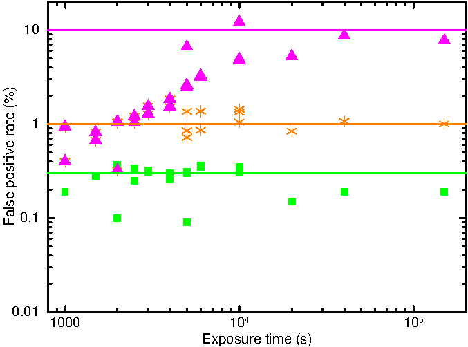
Fig. 7 False positive rate as a function of exposure time and flag. The green squares indicate ‘Good’ sources; the orange stars are ‘Good’ and ‘Reasonable’ sources, and the magenta triangles are ‘Good’, ‘Reasonable’ and ‘Poor’ sources.
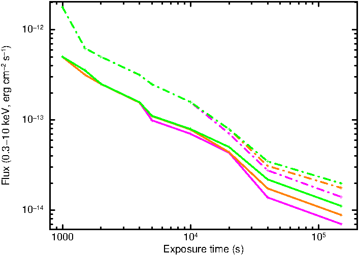
Fig. 8 Completeness of our detection system as a function of exposure time. The solid line indicates the level at which the catalogue is 50% complete, the dashed line, 90% complete. The green/orange/magenta lines refer respectively to good; good & reasonable; and good, reasonable & poor sources. For most exposures only the good line is visible for the 90% complete curve: this is because at the flux level at which the detection system is 90% complete, all detected sources are good.
6. Cross correlation with other catalogues.
We cross correlated our catalogue with various other catalogues, as listed below. We took a crude approach of simply listing all objects in the catalogue of interest that lay within 3σ of the X-ray source. Where more than one source per catalogue met these criteria all sources were recording, in increasing order of distance from the 1SXPS position. The catalogues we have correlated with in this way are:
- SDSS QSO DR5.
- XRT GRB catalogue.
- SwiftFT.
- 1SWXRT.
- 3XMM DR4.
- Rosat HRI.
- SIMBAD.
- XMM Slew Survey.
- Rosat PSPC.
- USNO-B1.
- 2MASS.
7. Catalogue Contents
There are four tables available for download. These are described in detail on the Table descriptions page.
- Sources
- This is the main catalogue table, the only one which is available in Vizier. This contains the details of the 151,524 unique sources in the catalogue.
- Detections
- This contains details of the individual detections in each dataset and energy band, of the sources.
- Datasets
- This contains details of the individual datasets (observations and stacked images) of which the catalogue is composed.
- Cross correlations
- This contains details of sources from external catalogues which are positionally coincident with 1SXPS sources.
8. Accessing and citing the catalogue
The catalogue can be downloaded as a FITS file, CSV file or SQL dump
or queried through this page. Not all columns contain values for each entry in the tables,
for example, in the Sources table, only source for which a spectral fit exists, have entries in the
Fitted* fields. In the CSV files, such empty entries are literally empty; in the FITS and SQL
files these entries are NULL.
If you use data from this catalogue in your work, please cite Evans et al. (2014) and in the acknowledgements section of your publication, please state:
This work made use of data supplied by the UK Swift Science Data Centre at the University of Leicester.
9. Changes
Changes made after the publication of the catalogue paper will be listed here.
UK Swift Science Data Centre
Last updated 2013 November 21
Web page maintained by Phil Evans
E-mail: swift help
Please read our privacy notice.