| site map

Home
About
The Swift Mission UK involvement Instruments
GRBs before Swift GRBs in the Swift era Non-GRB science with Swift GRB research at Leicester
Spacecraft status Swift in the press Swift Videos
Support
Helpdesk TOO requests Guest Investigator program Target visibility checker Search transient database
Data Access
Overview Quick Look GCN Notices Download obs data Search obs catalogue The 2SXPS catalogue The LSXPS catalogue
Data Analysis
Data analysis overview Swift software
Build XRT products
BAT data analysis guide XRT data analysis guide XRT digest UVOT data analysis guide
GRB Products
Full dataset Swift XRT products for GRBs XRT positions XRT light curves XRT spectra XRT GRB catalogue XRT GRB images Burst analyser Prompt dataset GRB field info XRT prompt analysis
Publications
Publication index Published papers Submitted papers XRT instrument papers ATels GCNs Conferences
Links
Databases NED Simbad GCN circulars archive GRB data table Software & Tools Swift Software (HEASoft) Xanadu WebPIMMS Institutional Swift Sites GSFC PSU OAB SSDC MSSL University of Leicester

Catalogue XRT results for GRB 091130B

Data were analysed using HEASOFT version 6.32

Summary Information

RA:	13h 32m 35.54s	LC breaks:	3
Dec:	+34° 05′ 19.7′′	LC type:	Canonical.
Err:	1.4′′	N_H,intr.:	2.01×10²¹ cm^-2
Gal long:	73.638	Redshift	Unknown
Gal lat:	78.748	Γ	2.3

Show light curve? | Show spectrum? | Show comparison with other bursts?

Jump to: Light curve | Spectra | Compare to other bursts.

If you use any of these data, please cite Evans et al. (2009), which describes how these products were created (see the usage policy for more information).

Light curve

Hide the light curve section.

This light curve comes from the light curve repository (if you use it, please cite Evans et al [2007, 2009]. Flares, marked by cross-hatched regions, are identified automatically, but may have been manually corrected. These are excluded from the fit. Any power-law breaks added to the fit must be required at the 4-σ level (according to an f-test) to be included in the best-fit. Details of all fits attempted are given below the plot. For more information see the light curve fitting documentation.

Fit Details

N_breaks	χ²	dof	Comments
0	1534	134
1	592	132	Break required. (5.08e-26 % probability of chance improvement)
2	362	130	Break required. (1.39e-12 % probability of chance improvement)
3	150	128	Break required. (3.91e-23 % probability of chance improvement). This is the best fit.
4	145	126	Break significance <4-σ (10.93 % probability of chance improvement)
5	138	124	Break significance <4-σ (3.73 % probability of chance improvement)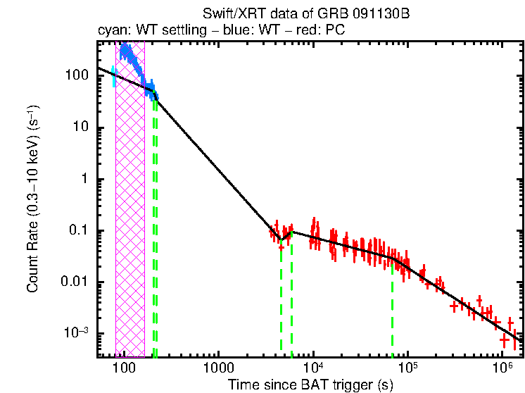

There are 1 flares excluded from the fit:

82.2—164 s

The best-fitting light curve has 3 breaks.

Click on the number of breaks in the table to the right to change which fit is plotted above and detailed below.

Currently showing the best fit.

α₁	0.78 (+0.11, -0.11)
T_b,1	206 (+9, -10) s
α₂	5 (+3, -3)
T_b,2	583 (+1.24 × 10³, -177) s
α₃	0.375 (+0.056, -0.124)
T_b,3	6.3 (+1.2, -2.0) × 10⁴ s
α₄	1.186 (+0.081, -0.115)

[Back to top]

Spectra

Hide the spectrum section.

Spectra have been created for each power-law segment in the best fitting light curve (shown above). Times of flaring have not been removed, however this makes little difference to most spectra (see Fig 7/8c of Evans et al. 2009). For more information see the time-resolved spectroscopy documentation.

Jump to: phase1|phase2|phase3|phase4

phase1 spectrum (T0 + 91 to 206 s)

Download spectral files for phase1 spectrum.

Plots to download

WT mode. Mean photon arrival: T0+127 s

N_H (Galactic)	8.25 × 10¹⁹ cm^-2
N_H (intrinsic)	3.02 (+0.26, -0.25) × 10²¹ cm^-2
z of absorber	0
Photon index	2.01 (+0.06, -0.06)
Flux (0.3-10 keV) (Observed)	5.21 (+0.18, -0.17) × 10^-9 erg cm^-2 s^-1
Flux (0.3-10 keV) (Unabsorbed)	7.77 (+0.22, -0.24) × 10^-9 erg cm^-2 s^-1
Counts to flux (obs)	3.62 × 10^-11 erg cm^-2 ct^-1
Counts to flux (unabs)	5.40 × 10^-11 erg cm^-2 ct^-1
W-stat (dof) What's this?	608.19 (618)
Spectrum exposure	114 s

[Back to top]

phase2 spectrum (T0 + 206 to 231 s)

Download spectral files for phase2 spectrum.

Plots to download

WT mode. Mean photon arrival: T0+217 s

N_H (Galactic)	8.25 × 10¹⁹ cm^-2
N_H (intrinsic)	2.8 (+1.0, -0.9) × 10²¹ cm^-2
z of absorber	0
Photon index	3.1 (+0.4, -0.4)
Flux (0.3-10 keV) (Observed)	7.58 (+1.07, -0.92) × 10^-10 erg cm^-2 s^-1
Flux (0.3-10 keV) (Unabsorbed)	2.34 (+1.37, -0.30) × 10^-9 erg cm^-2 s^-1
Counts to flux (obs)	2.23 × 10^-11 erg cm^-2 ct^-1
Counts to flux (unabs)	6.87 × 10^-11 erg cm^-2 ct^-1
W-stat (dof) What's this?	151.21 (167)
Spectrum exposure	25 s

[Back to top]

phase3 spectrum (T0 + 3492 to 62950 s)

Download spectral files for phase3 spectrum.

Plots to download

PC mode. Mean photon arrival: T0+26570 s

N_H (Galactic)	8.25 × 10¹⁹ cm^-2
N_H (intrinsic)	1.9 (+0.4, -0.4) × 10²¹ cm^-2
z of absorber	0
Photon index	2.25 (+0.15, -0.14)
Flux (0.3-10 keV) (Observed)	1.60 (+0.13, -0.11) × 10^-12 erg cm^-2 s^-1
Flux (0.3-10 keV) (Unabsorbed)	2.46 (+0.17, -0.17) × 10^-12 erg cm^-2 s^-1
Counts to flux (obs)	3.06 × 10^-11 erg cm^-2 ct^-1
Counts to flux (unabs)	4.72 × 10^-11 erg cm^-2 ct^-1
W-stat (dof) What's this?	267.43 (347)
Spectrum exposure	26.4 ks

[Back to top]

phase4 spectrum (T0 + 62950 to 1381667 s)

Download spectral files for phase4 spectrum.

Plots to download

PC mode. Mean photon arrival: T0+277539 s

N_H (Galactic)	8.25 × 10¹⁹ cm^-2
N_H (intrinsic)	2.4 (+0.7, -0.6) × 10²¹ cm^-2
z of absorber	0
Photon index	2.30 (+0.22, -0.20)
Flux (0.3-10 keV) (Observed)	1.55 (+0.17, -0.15) × 10^-13 erg cm^-2 s^-1
Flux (0.3-10 keV) (Unabsorbed)	2.59 (+0.25, -0.25) × 10^-13 erg cm^-2 s^-1
Counts to flux (obs)	3.05 × 10^-11 erg cm^-2 ct^-1
Counts to flux (unabs)	5.09 × 10^-11 erg cm^-2 ct^-1
W-stat (dof) What's this?	301.75 (288)
Spectrum exposure	181.3 ks

[Back to top]

Comparison with other bursts

Hide the comparison section.

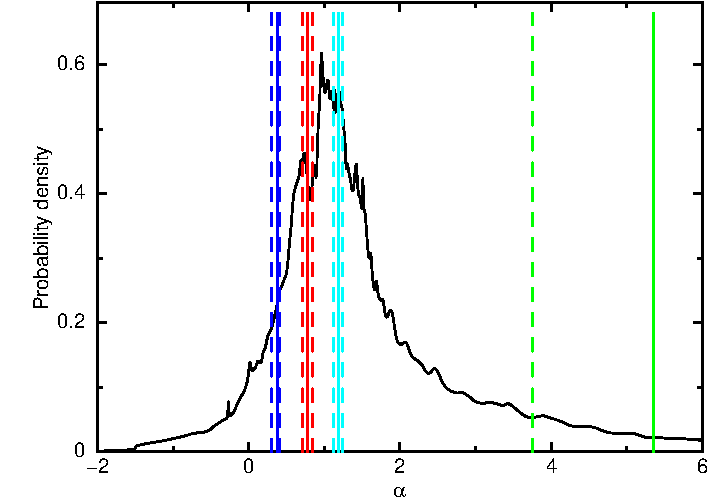
Parameter distributions

The plots below show the probability density functions of the temporal and time-averaged spectral parameters for all GRBs, with the data for GRB 091130B shown on in colour. Click the images for larger versions.

For all plots, the solid vertical lines mark the values for this GRB, and the dashed lines the 1-σ uncertainties. For α and T_b, the colour changes for each phase. For the spectral parameters, the WT fits are shown in blue and the PC in red. These figures correspond to Figs. 5,6, 7a and 8a of Evans et al. (2009). See the PDF documentation for more information.

Temporal indices	Break Times	N_H	Spectral indices

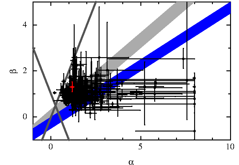
Closure Relationships

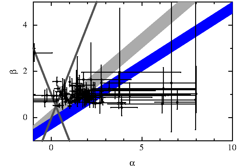
The plots below show (α, β) scatter plots for each phase of all Canonical light curves. GRB 091130B is shown in colour; where multiple points appear in a given phase (e.g. WT and PC mode spectra for that phase), the different colours refer to different spectra. α and β are the temporal and spectral energy power-law indices respectively. The shaded regions mark those allowed by the standard closure relationships. These figures correspond to Fig. 10 of Evans et al. (2009). See the closure relationship documentation for more information.

Canonical Steep phase	Canonical Plateau	Canonical 'Normal'	Canonical Post jet-break

[Back to top]