- Home
- About
- Support
- Data Access
- Data Analysis
- GRB Products
- Publications
-
Links
Databases NED Simbad GCN circulars archive GRB data table Software & Tools Swift Software (HEASoft) Xanadu WebPIMMS Institutional Swift Sites GSFC PSU OAB SSDC MSSL University of Leicester
Swift-XRT GRB light curve Repository — Online Documentation
Contents
- Summary
- Using these light curves
- Per-GRB light curve pages
- Rebinning the data
- New bursts
- When new GRB data arrive
- Changelog
Summary
This web site provides a repository of Swift-XRT light curves and hardness ratios for every GRB this instrument has detected. There are four ways provided of selecting a GRB to view: a page of thumbnail images for each GRB, a search box (where you can enter a GRB number, or BAT trigger number), a year/month menu and a panel showing the 5 most recently observed GRBs. Each of these links to the light curve page for that burst.
Bursts which the XRT did not observe or did not detect do not have thumbnail images, even if they are Swift-detected bursts.
The process of light curve creation is described in full in two refereed papers: Evans et al. (2007, A&A, 469, 379) and Evans et al. (2009, MNRAS, 397, 1177). Most of the questions we are commonly asked about the light curves can be answered by looking at these papers. An overview of the algorithm is also given online.
Back to contents | Back to repository
Using these light curves
The data available from this repository are available for use in research and publications, provided that this is acknowledged. We request two forms of acknowledgement. Where the data are first introduced, please cite Evans et al. (2007, A&A, 469, 379) and Evans et al. (2009, MNRAS, 397, 1177) which describe how the data were produced. In the acknowledgements section, please use the following text:
This work made use of data supplied by the UK Swift Science Data Centre at the University of Leicester.
Back to contents | Back to repository
Per-GRB light curve pages
When you select a GRB, you will be taken to the light curve page for that burst, which is described here. (For details of how these products are created see Evans et al [2007, 2009], and the changelog on this page). An overview of the algorithm is also given online.
Overview
The page begins with a title, and then indicates which dataset triggered the most recent update of the light curve. This is followed by a series of links to any other products which exist for this burst, to the rebin interface and this documentation page; and a warning if data for this GRB are still on the quicklook site (i.e. more observations may be forthcoming).
If any data points had to be flagged as unreliable, this is reported next, along with a control to allow those data points to be shown. Unsafe data points are described below.
The light curves are shown next, presented first in graphical format. There will be (up to) four plots, all of which link to the ASCII data from which they were created. Each light curve also comes with a link to allow the plot to be rescaled, and may also include the controls to toggle whether WT-mode systematic errors are included. Finally, links are provided to allow the download of the various files available in the light curve repository for this GRB.
Back to contents | Back to repository
Light curves and downloads
There are up to four light curves available to view and download, followed by a list of up to 18 files. The images are:
- Flux light curve (where available)
- The count-rate light curve (described next) converted to observed 0.3—10 keV flux using a constant Energy Conversion Factor (ECF). The ECF is derived for each GRB individually, using the automatic fit in the spectrum repository. Since only a single ECF is used per burst, the effects of spectral evolution are not included in this light curve, for datasets which include spectral evolution, see the Burst Analyser.
- Count-rate light curve
- A light curve showing the source count rate, after the background has been subtracted and corrections for pileup, bad columns, and the size of the source-data extraction region have been applied.
- Detailed light curve
- As above, but with the background level shown on the same plot (note that at low count rates, the net source count rate can lie below the background rate but still be a 3-σ detection). The fractional exposure is also shown, in the bottom panel.
- Hardness ratio
- Similar to the basic light curve, but in two bands: 1.5—10 keV and 0.3—1.5 keV. The bottom panel is the ratio: hard/soft.
The links at the foot of the page include postscript versions of all of the plots, the ASCII versions (which can also be reached by clicking on the images), and various other files which are described under File formats and contents below.
WT settling mode data
As of 2009 July, Swift-XRT collects data in WT mode while slewing. These data are only usable for bright objects, such as newly-discovered GRBs, but they enable us to begin collecting the critical early data a few seconds earlier. These ‘settling mode’ data points are shown in cyan on the light curve plots.
In order to produce a correct light curve, knowledge of the GRB position in the XRT coordinate frame is critical (this is discussed in detail below). While Swift is still slewing the spacecraft attitude information can be inaccurate, and the degree and direction of the inaccuracy is a function of time. This was responsible for the artifacts previously seen in settling mode data. For bright GRBs it is possible to perform high-cadence centroiding within the WT-mode window to track the position of the GRB within the XRT co-ordinate frame. In this case the settling mode data can be correctly analysed. For fainter bursts, the centroiding cannot be performed with sufficient cadence (roughly every 0.2 s), and therefore the settling mode data are rejected until the slew rate has fallen to around 20″/sec, at which point the attitude information tends to stabilise. For bursts which are fainter still, it may be impossible to determine the GRB position within the XRT frame at all; in those cases the settling mode data are not included in the light curve.
Back to contents | Back to repository
Changing the plots
There are up to three ways in which you can manipulate the plots shown, which are described below. If the light curve includes WT mode data then you can toggle whether the systematic errors are shown, and if there are ‘unreliable’ data points then you can select whether or not to show them. These controls affect all plots on the page simultaneously, and also the ASCII file linked to by the plots. You can also rescale the plots, that is, change the axis limits and regenerate the graphical image of the light curve.
WT-mode systematic errors
WT-mode data are subject to extra uncertainties in addition to the statistical errors, when the GRB is near to the bad columns on the CCD or the edge of the field of view, or the data are piled up. This uncertainty is understood and calibrated, and we add an error to each WT-mode data point which reflects this. For simplicity, we refer to this as a systematic error, that is, it reflects an uncertainty in the absolute flux level of the object (a DC offset). This error will be different each time the spacecraft slews to the object, so the systematic error should be considered when comparing the flux level of an object in one snapshot with that in another (of course, since we have calibrated this as a 1-σ error, it is expected that for a constant source, 1 in 3 snapshots will not be consistent with the rest). In reality, the error is not always systematic in nature but can vary in magnitude between bins in the same snapshot, therefore whether this error should be taken into account should be decided on a case by case basis, as we now explain.
The systematic error is caused by inaccurate knowledge of the GRB position on the XRT CCD, and is a calibrated quantification of the uncertainty caused by this inaccurate knowedge (full details are at the end of this section). So if the GRB maintains a constant position on the CCD, this error is purely systematic: all datapoints in a snapshot are affected in exactly the same way. Therefore in this case, the systematic error should not be considered when evaluating point-to-point variation within a snapshot, otherwise the significance of such variation will be underestimated. On the other hand, if the object is moving on the CCD, the ‘systematic’ error may be variable within a snapshot. For example, if our measurement of the GRB position on the CCD is incorrect by one pixel, but the GRB is 5 pixels from the bad columns, then the systematic error caused by the poor position is small; but if the spacecraft moves such that the GRB drifts onto the bad columns, then the systematic error will get larger as the GRB moves towards and onto the columns. In this case, the variation between the bins within that snapshot is being exaggerated by the poor positional information, and therefore the ‘systematic’ error should be used when considering the significance of those variations.
The practical impact of this is that, in order to evaluate the significance of intra-snapshot variability, one must check whether the source position within the CCD is stable. Since in WT mode only 1-dimensional position information is available, only DETX position variations need considering. On the light curve pages a link is provided above each light curve, entitled, ‘View systematics and position variation’. This opens up a plot showing the DETX position of the object and the fractional systematic error, as a function of time. This can be used to decide whether or not the source remains in a stable position during the time interval in question (this plot can also be rescaled to zoom in on a specific time range. An example is given in Fig. 1. During times where the DETX position is varying (within a snapshot) the systematic error should be taken into account when assessing source variability; during times where DETX is constant, the systematic can be safely disregarded, for the evaluation of source variability within the snapshot. At all times, when determining the absolute flux level, the systematic should be included.
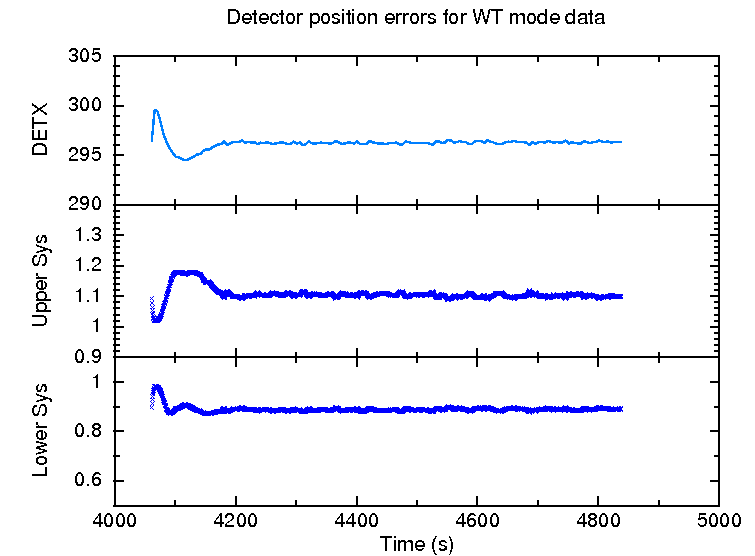
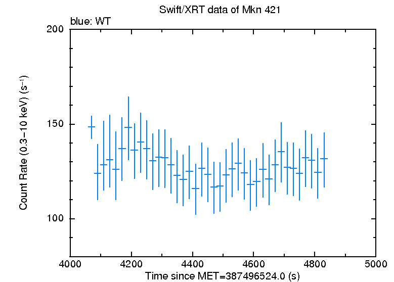
Fig. 1. Left: An example of position variation and the resulting systematic error factors. This shows one snapshot in which the object moves significantly on the CCD which, due to the proximity to the bad columns, causes significant uncertainty at early times. Thus the variation seen in the light curve (right) at the start of the snapshot should only be interpreted when the systematic errors are included.
As Fig 1 shows, the systematic error plotted is actually a factor, since (see below) it is really an uncertainty in the PSF correction factor that is applied to the light curve.
By default, the systematic error is included in the light curves on the repository, however by deselecting the check box above the light curve, these can be turned off. Note that the checkboxes are linked, so clicking on any of them toggles the inclusion of systematic errors for all of the plots on the page. If the GRB is not piled up or near the bad columns or field-of-view edge, then the systematic errors are negligible, and toggling this box will make no difference to the light curves.
More detail: The need for, and determination of, the systematic error
The systematic errors arise in cases where some of the events from the source are lost, either because they lie over the bad columns or outside the field of view, or because the core of the PSF had to be excluded because of pile up. In each of these cases, when the light curve is constructed the instrumental PSF is used to calculate the fraction of events that were lost, and the count-rate is multiplied by the corresponding correction factor. However, in order to do this calculation correctly, the position of the source on the XRT CCD must be known accurately. For example, if it is believed that the wings of the PSF are over the bad columns such that only 2% of the flux is lost, whereas in reality the source is much closer to those columns and 30% of the flux is lost, then the correction factor will be far too small and consequently the light curve bins at those time will report a spuriously low count-rate. Or, in the case of pile up, if we believe we are excluding the central 4 pixels of the PSF, but actually the annulus is not correctly centred on the source, then the correction factor will clearly be wrong.
To solve this problem, we use PSF centroiding once per snapshot to determine the position of the GRB in the XRT's RA/Dec coordinate frame. This may not be the same as the ICRS RA/Dec system, due to uncertainties in the spacecraft attitude, hence the need to centroid repeatedly. Although it is the CCD position we are interested in, we need to centroid in RA & Dec, because Swift does not remain stationary while on target, but moves slightly, thus the PSF in the raw CCD images becomes smeared. The spacecraft attitude information corrects for these movements, making the PSF well defined and stable in the RA & Dec frame (although there is a 3.5″ systematic uncertainty associated with Swift's absolute attitude, the relative attitude information appears to be stable within an orbit. That is, the size and direction of the small movements Swift makes while pointing are well described in the attitude files.). We then use the attitude information from the spacecraft to convert the RA & Dec of the GRB into a CCD-coordinate position as a function of time. The uncertainty in the PSF centroiding is well constrained as a Gaussian with σ=0.64 pixels. Similarly the WT mode PSF is known, as is the location of the bad columns, and the box or box annulus within which source events are collated. Therefore, for a given measured CCD position, we can work out the probability of the GRB really being at any true CCD position, and how wrong the measured count-rate would be given that combination of measured and true positions. Integrating this over the Gaussian uncertainty in the centroiding output allows us to produce a systematic error in the correction factor as a function of the measured CCD position of the GRB, this is shown in Fig. 2. If this error in the correction factor is Ecf, then the error in the count-rate caused by the centroiding inaccuracy is Ecf(R-1), where R is the measured (uncorrected) count-rate. This can then be added in quadrature to the statistical error on the count-rate. The plot below shows the fractional error as a function of measured position on the CCD. As can be seen, this is slightly asymmetric, so the errors on the final light curve are also asymmetric.
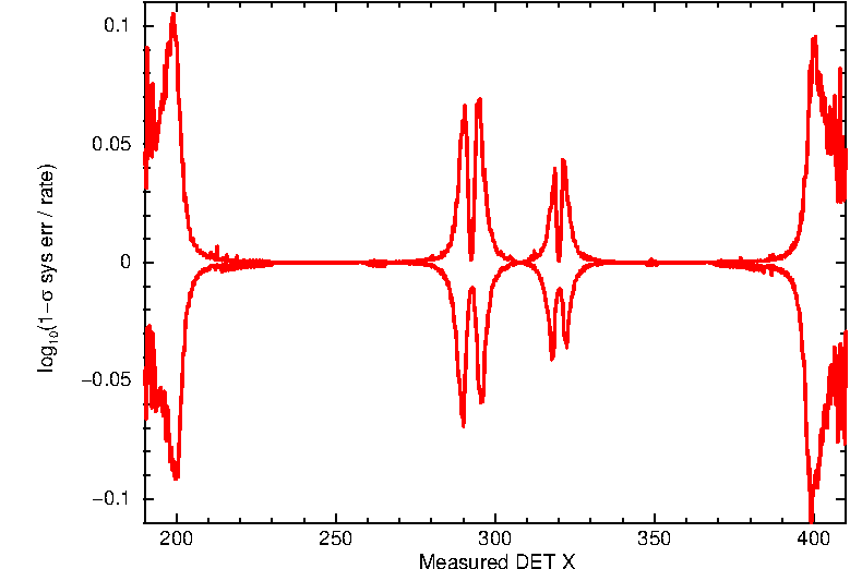
Fig. 2 The 1-σ fractional systematic error as a function of the measured position of the GRB on the CCD. The upper and lower curves show the positive and negative errors respectively.
Unreliable data points
If the position of the object within the XRT CCD is not known, the count-rate may be unreliable. In part, this is due to the issues described above, but also of course, even in the absence of bad columns and pile up, the source extraction region needs to be centred on the source. As the XRT astrometry has a nominal accuracy of 3.5″ (90% confidence), the light curve software attempts to centroid on the object for each snapshot. In any case that a centroid cannot be found, or is more than 12″ in WT mode / 20″ in PC mode from the best-known GRB position, that best-known position is used, data from that snapshot are considered unreliable.
If unreliable data are found, a warning appears at the top of the results page to warn of this fact, give some information about the affected times, and a control is provided to toggle whether those data are included in the light curve. Note that “unreliable” does not mean “wrong” and in many cases the data will be reliable, it is only if the spacecraft astrometry is particularly bad that a problem is expected: the toggle switch is to draw your attention to the questionable data so that outlying values caused by bad centroids can be spotted.
Rescaling light curves
Before each of the light curve images is a link inviting you to "rescale" the light curve. This opens a new panel from which you can choose the axis limits, and whether they are linear or logarithmic, and then replot the data. Note that, unlike rebinning this does not change the data, only the visualisation.
Back to contents | Back to repository
File formats and contents
The light curve images all serve as links to the data file from which they were produced, the formats of these files are discussed below. After the images there is a series of links to different files which are not plotted, but contain more information. The formats of these files are also given below. Note that whether or not the light curve data includes systematic errors and the bad WT points depends on the settings of the controls, described above.
The Basic Light Curve
The Basic Light Curve shows the count-rate as a function of time. The related ASCII file is ready for use in QDP, thus begins with a READ TERR line (to tell qdp which columns contain errors) There are 6 columns in this file, which are:
- Time
- Time -- positive error
- Time -- negative error
- Source count rate
- Positive error in count rate (1-σ)
- Negative error in count rate (1-σ)
There are up to five datasets in the file, separated by a line of NO NO
NO NO NO, (again, for compatibility with QDP). The datasets appear in
the following order: Windowed Timing (WT) settling mode data, WT data; WT upper limits; Photon
Counting (PC) data; PC upper limits. Depending on the object, some of these may
be missing, however each dataset begins with a comment (denoted by a leading
!) identifying it.
The Detailed Light Curve
The Detailed Light Curve contains the information from the Basic Light Curve and also the background level in the top panel. The lower panel shows the fractional exposure in each bin. Note that the background level is the expected background rate in the source region, however as the source region is dynamic (it is smaller when the source is fainter) some correlation between source and background count-rates is expected.
The columns in the ASCII file are the same as for the basic light curve, however
there are more datasets (again separated by lines of NO entries): the count-rate, upper limits
(if applicable), background level and fractional exposure; first for WT mode then PC mode.
Note that the WT settling mode data do not appear in here since all settling mode data
points have a fractional exposure of 1 and the background rate is negligible.
The Hardness Ratio Light Curve
The hardness ratio plot contains 3 panels, showing the hard-band data in the top panel,
the soft-band data in the middle, and the hardness ratio in the bottom panel. The hardness
ratio is defined as Hard/Soft. By default the hard and soft bands are 1.5—10 keV and 0.3—1.5 keV
respectively, although if you rebin the light curve you can change these
values.
The hardness ratio ASCII file again contains the same basic 5 columns as in the basic light curve, with three datasets: hard band data, soft band data and hardness ratio, per instrument mode (WT settling mode, WT mode, PC mode).
Detailed data downloads
The files below the images comprise postscript versions of each light curve, per-mode light curves (referred to as the basic data), a detailed dataset per mode and event lists. The basic data are the same format as the basic light curve, whereas the detailed data contain many more fields, giving all available information about each bin. The columns in the detailed files are:
- Time
- Time -- positive error
- Time -- negative error
- Net source count rate
- Positive error in the above (1-σ)
- Negative error in the above (1-σ)
- Fractional exposure
- Background rate
- Error in background
- Total correction factor
- Total counts measured in the source region
- Expected number of background counts in the source region
- Exposure time in the bin (i.e. bin width * fractional exposure)
- Detection significance in this bin
- Signal-to-noise ratio in this bin
- The fractional systematic error in the negative direction (WT only)
- The fractional systematic error in the positive direction (WT only)
The "total correction factor" is the ratio of the corrected count rate to observed count rate in this bin. The corrected count rate has been amended to account for: bad pixels/columns, field of view effects, pile-up and source counts landing outside the extraction region.
Sigma is the detection significance of the source in this bin (=net counts/error in bg counts for a frequentist bin. For a Bayesian bin it is the confidence level at which the source count rate is above 0). For an upper limit, the value written is the detection significance of the data which were replaced with the limit. The upper limit is at the 3-σ level for GRBs, and is calculated using the Bayesian method (see Kraft, Burrows & Nousek, 1991, ApJ, 374, 344).
The signal-to-noise ratio is simply the count-rate divided by its negative error.
The fractional systematic error is the multiplicative component of the error which reflects
the systematic errors related to position uncertainty.
For example, in the positive direction, if Eup is the extra error component,
and Rmax is the 1-σ upper bound on the count-rate value including this component:
Eup = Rmax - R
= R*S -R
= R (S-1)
where R is the count-rate in the bin, and S is the fractional systematic error in the positive direction, and
E is the resultant systematic error which has to be added in quadrature to the statistical error on the count rate
to give the final error. If the ‘Include systematic errors?’ check-box is selected, the count-rate error
already includes this component.
Event lists
The event lists (source and background for each mode), contain all
source or background events selected during the light curve creation. As well as the
standard columns (TIME, position information, energy etc), the following
information has been added:
- SRCRAD - Source extraction region radius (pixels).
- PUPRAD - Radius excluded due to pileup (arcseconds) - source event lists only.
- SRCAREA - Area of the source extraction region (square pixels) - background event lists only.
- BGAREA - Area of the background extraction region (square pixels) - background event lists only.
Back to contents | Back to repository
How to rebin the data
When binning the GRB light curves, the software applies 5 criteria to determine whether a bin is complete. These are:
- There must be at least X counts in the source region.
- The bin must be at least Y seconds long.
- The bin must use all events from a given CCD frame.
- The source count rate must be at least Z-σ above the background.
- The signal-to-noise ratio must be at least Q.
The variables given above as X, Y, Z, Q can all be adjusted via the rebinning interface. Criterion 3 is a little obscure: since the data are read out at discrete times, one can get many events with the same timestamp. Criterion 3 ensures that these events are all put in the same bin, to prevent overlapping error bars.
In the standard products, the data are binned dynamically; that is, the
binning criteria vary with count rate. This has been found to be the optimal
way of binning GRB data, where the flux can vary by more than five orders of magnitude
across the light curve, and a single binning approach is not optimal.
X, the minimum number of counts in a bin, is valid at a count rate of
1 count per second (cps); when the count rate changes by some factor (the
rate factor), X changes by some other factor (the bin
factor). The default values for these factors are 10 and 1.5
respectively, thus an order-of-magnitude change in count rate produces a
factor of 1.5 change in bin size. This is done discretely rather than
continuously, so if X=20 then where the count rate lies in the
range 1-9.99 cps a bin must contain at least 20 counts. However, when the
count rate is 10-99.99 cps, there must be 30 counts for a bin to be full. At
lower rates of 0.1-0.99 cps, only 13 (=20/1.5) counts are needed to complete a
bin, although this is rounded to 15: no matter how low the count rate goes, a
bin will always need at least 15 counts, to ensure that using Gaussian methods
to propagate errors statistics is valid.
While the above approach gives useful, usable results for almost all GRBs, it may not give the best possible results for a given burst. We have thus provided an interface to allow the user to rebin the light curves for themselves.
From the light curve page for your GRB, follow the "Rebin this light curve" link. The form with which you are presented contains the fields detailed below. If you have javascript enabled, clicking on the field name will open a help box with more information about that field.
The first option is the Binning Method. There are four ways of binning the data:
- Counts
- the standard GRB-type binning, defined by the criteria described above.
- Time
- bins of fixed duration.
- Snapshot
- One bin is produced for each observing snapshot.
- ObsID
- One bin is produced for each obsID.
The following options are available for all four binning methods:
- Minimum sigma:
- The minimum significance a bin must have to be considered full. Significance refers to the probability of the measured count-level being a fluctuation in the background, given in Gaussian σ (e.g. ‘3’ means that there must be a <0.3% probability of getting the detected number of events in the bin, given the backround level). If a bin is below this significance then, for counts binning, it will not be considered full; for other binning methods, an upper limit at this significance level will written instead of the measured count-rate, if upper limits are enabled.
- Allow upper limits
- Whether bins can contain an upper limit if the detection significance falls below the minimum sigma, or not. This can be set for PC and WT modes separately.
- Allow Bayesian bins
- Whether the count-rate can be calculated using a Bayesian method (see Kraft, Burrows & Nousek, 1991, ApJ, 374, 344) when they fall below some threshold. This can be set for PC and WT modes separately. The thresholds are given below.
- When to use Bayesian statistics
- If Bayesian bins are enabled, these will be used when a bin contains fewer than some specified number of counts, or the signal-to-noise ratio of the bin falls below a specified level. These fields allow you to specify those levels.
- Energy and grade selection:
- The default is to use the same energy and grade ranges which were used for the light curve you are rebinning (the standard light curves all use 0.3-10 keV for the main light curve, 0.3-1.5 keV and 1.5-10 keV as the soft and hard bands respectively, and grades 0-12). You can select "User-specified" here, allowing you to set these fields yourself.
The following fields are only available if you have chosen "User specified" for the energy and grade selection.
- Energy range for main curve:
- Only events with energies in this range will be included in the light curves.
- Grade range for main curve:
- Only events with grades in this range will be included in the light curves.
- Soft energy band:
- The range of energies to use in the soft band for the hardness ratio. Note, these energies must lie within the range for the main curve.
- Hard energy band:
- The range of energies to use in the hard band for the hardness ratio. Note, these energies must lie within the range for the main curve.
The following options are available only for the Counts binning method:
- Counts per bin:
- The minimum number of counts needed for a bin to be complete (criterion 1 above). Must be specified for WT and PC mode.
- Minimum bin length:
- The minimum duration required for a bin to be complete (criterion 2 above). Must be specified for WT and PC mode.
- Dynamic binning:
- Whether to use dynamic binning (see above).
- Rate/bin factor:
- These two boxes control the dynamic binning (if selected), full details are above.
- Minimum counts per bin:
- Dynamic binning cannot reduce the minimum counts per bin indefinitely. This defines the "hard" minimum, i.e. regardless of dynamic binning there must always be at least this many counts. We recommend that this is at least 15, to ensure that the Gaussian error propagation is valid.
- Minimum SNR per bin:
- The minimum signal-to-noise ratio (SNR) that a bin must have to be considered full (criterion 5 above). SNR is defined S/σS, where S and σS are the number of source counts and the error thereon respectively.
- Maximum orbital gap
- The maximum gap between orbits (or obsIDs) which a bin can span, in seconds. Once a bin encounters a gap longer than this, it will be saved, even if it does not meet the criteria to be considered full.
The following options are available only for the Time binning method:
- Bin length
- The size of the bins required for the light curve
- Hardness ratio bin length
- The size of the bins required for the hardness ratio light curve
The snapshot and obsid binning have no special options to set.
Once you are happy, click "Rebin data". You will be redirected to a "holder page" which will auto-reload every 10 seconds until the process is finished, at which point it will be replaced with the light curve page. Note: your rebinned light curve will be stored at a temporary URL, and deleted after 24 hours. There is no link to it, so it is a good idea to bookmark the holder page when the rebin process starts, so that you can find the page again.
Back to contents | Back to repository
New Bursts
When a GRB is detected by the Swift-BAT, or a ToO for a GRB detected by another mission is uploaded, the UKSSDC servers automatically register the object for analysis. The arrival of data on our quicklook site automatically triggers the the GRB analysis software. This first reprocesses the XRT data with the most recent version of the Swift software and then constructs the high-level products such as the light curve.
Back to contents | Back to repository
Updating the data
The update procedure is almost identical to the new burst procedure. It is triggered by the arrival of new data, and again runs after those data have been locally reprocessed. When a light curve is updated it is not ordinarily completely rebuilt. Instead the time of the start of the final hardness ratio bin is determined, all existing data after this point are deleted, and the update begins at this time. There are two exceptions to this: if older data are also received (sometimes data are not delivered in "order"), or if the light curve was previously built before any PC mode data had arrived, but PC mode data are now available. The reason for the latter is that, without PC mode data, we cannot determine the most accurate XRT position of the GRB so the light curve is built using the position from the prompt data analysis. As soon as PC mode data are available a better position is available and should be used.
Back to contents | Back to repository
Swift software versions
We endeavour to ensure that the GRB products provided on this website are created with the most up-to-date version of the Swift software and calibration. After a new version is released, there will be a short period of time while we test this software and confirm that our codes still work as expected, and then we will reprocess all of our online products using the new software/calibration. This will ordinarily be done offline, and then the products updated en masse, rather than piece aat a time.
Changelog
The light-curve generation software is occasionally modified. Any changes are listed here.
- 2014 October — Several changes implemented:
- Systematic errors are now added to WT mode data, reflecting the effect of uncertainty in the correction factor caused by position uncertainty. Controls are provided to toggle whether these errors are plotted. See the WT systematics section for details.
- Where the source cannot be accurately localised in the WT mode data, the data are rejected by default. Controls are provided to show these points. See the Unsafe WT-mode Points section for details.
- Handling of the settling mode data problem previously reported is improved so that, for brighter bursts, the full settling mode data can be used. Details on this are in the Settling data section.
- The detection of sources in the background is now performed only once, at the start of the light-curve build, and uses all available data. Sources found at this time are then excluded from the background region in all observations (previously the check for background sources was conducted on each obsID separately).
- Minor efficiency changes have been made to make the code run faster, without changing the algorithm.
- 2014 March 14 — many light curves show settling mode data (the early, cyan points, showing data taken while the spacecraft was still moving) which appear to indicate a rapid flux decline that we do not believe to be real. We have identified the cause of this problem, related to uncertainties in the spacecraft attitude as it slews. For now, data which are affected by this problem are excluded. We are investigating whether it is possible to retrieve information from these data, and a further update will be forthcoming if this is successful.
- 2014 February 24 — a bug was fixed which sometimes caused light curves of off-axis sources to fail to be created.
- 2014 January 13, Binning code rewritten:
We have re-written the code that bins the light curves, making it much quicker and memory efficient, correcting an important issue, and giving a few new options to the user. Full details are available at this page, or a summary is given here:- The bad-column correction is now calculated with high cadence, to correct for the pointing instability issues that occasionally arise.
- For WT mode data the position of the source on the XRT image is determined via a PSF fit, rather than extrapolated from the PC-mode position.
- Support exists for different Swift attitude files.
- Time-resolution of WT mode pile-up management is improved.
- In GRB-binning there is now a minimum signal-to-noise ratio requirement needed for a bin to be considered full.
- You can allow bins to be upper limits or to use Bayesian statistics when they drop below some threshold.
- The maximum size of a bin can be specified when using the GRB-like binning.
- The maximum gap in observations over which data can be carried can be specified when using the GRB-like binning.
- The way observing gaps are handled by the binning has been improved.
- The binning (and rebinning) process runs much faster and more memory efficiently.
- 2010 January 5, WT settling mode data:
In 2009 July the collection of data in WT mode during spacecraft slews was enabled. This allows us to record data on a new GRB as soon as it enters the XRT WT-mode field of view (the "settling" phase), usually 10-20 s before the standard pointing-mode datasets. As of 2010 January 5th existing light curves have been updated to use these data where available, and all GRB light curves will also include these new data -- provided at least 15 source events were detected. There is a short (~10 s) gap between the end of the settling- and pointing-mode datapoints; this gap occurs as the XRT takes initial images to try to find the GRB in the onboard software.
During the spacecraft slew the attitude information is less accurate than when the spacecraft is pointing, thus bad column and pileup corrections in the settling-mode data have a 20% systematic which is included in the datapoint errors in the automatic light curves. WT settling mode data are binned in the same way as pointing mode data, and for rebinned light curves the binning settings supplied for WT mode data are applied to pointing and settling mode data alike. - 2009 November 4 - A new centroid now is determined for each snapshot with more than 40 source counts. If the source is fainter than this the exposure-weighted mean position determined so far is used. This improves light curves in the rare cases where the attitude information is of low accraucy. A second change was made at the same time, whereby the definition of the PSF wings used for pileup determination is brightness dependent. This improves pile-up correction in very bright sources (e.g. GRB 090904A, where the XRT was in PC mode while the source was 100 counts per second).
- 2009 May 07: Several minor tweaks, the most important of which affects some upper limits. The others
make almost no noticeable changes to the light curves.
- Bad pixel correction factors for upper limits are no longer taken as the average of the correction factors of the source events (as for full bins) but as the average of the correction factor for each snapshot in the upper limit.
- The error on the background rate is now correctly calculated; previously it was slightly overestimated.
- The source and background regions now have their areas corrected for bad columns, rather than assuming, a fully-exposed circle or annulus.
- The x-axis for non-GRB object plots has been widened so that the first and last points are not on top of the axis box.
- 2008 October 06: Three minor changes have been made, which have a small effect on a small (<10) number of
light curves:
- The position of the GRB on the XRT is now found using a PSF fit (see Goad et al. 2007), rather than xrtcentroid. This means the position is correct even when the GRB is near the bad columns.
- The pile-up detection has been modified -- if the uncorrected count-rate exceeds 0.9 counts per second at all, but the PSF fit shows no evidence for pileup, an annulus with an inner radius of 2 pixels is used anyway.
- Where pileup has occurred, we use xrtmkarf to determine the pileup (and bad column) correction factors. Where pileup has not occurred, we still numerically integrate the PSF to determine the bad column correction. This has improved the pile up correction for 4 GRBs.
- 2008 Jul 30: Three minor changes concerning the binning have been made and
reapplied retrospectively to all GRBs.
- A minor bug in determining the range of each bin was fixed -- a GTI devoid of events lying between bins may not previously have been correctly included. Comparing the corrected curves with the original ones shows that a tiny fraction of a percent of bins were affected by this; the change affects neither large nor small-scale structure of the light curves.
- The bin centroid was previously defined as the mean photon arrival time within the bin; this has been amended to the mean logarithmic photon arrival time. This gives a better indication of when most photons arrives in a bin.
- We have changed the way 'spare' counts at the end of a snapshot are handled, to reduce occurrences of long bins with very low fractional exposure. Previously, counts not in a bin by the end of a snapshot were added to the previous bin if there had been one this snapshot, and otherwise carried forward. Now, these 'spare' counts are only carried forward if either there have been no bins yet for this XRT mode in the light curve, or if the start of the next snapshot is closer in time to these counts than the end of the last bin. Otherwise, the counts are appended to the previous bin, even if that occurred several snapshots ago, since this gives a higher fractional exposure to the bin.
- 2007 Jun 18: If the final datapoint has fewer than 15 counts, do not automatically replace it with an upper limit. First, use Bayesian statistics to find a 3-σ error on the count-rate. If the lower limit of this is non-zero, calculate the 1-σ error using the Bayesian method, and plot this point as a bin, otherwise plot an upper limit. NOTE: If the bin contained fewer than 15 counts, future counts will still go into this bin, rather than forming a new bin.
Back to contents | Back to repository
UK Swift Science Data Centre
Last updated 2014 October 7
Web page maintained by Phil Evans
E-mail: swift help
Please read our privacy notice.