Contents
- Overview
- Results pages
- -Creation algorithm
- -Caveats and checks
- When are products built?
- Usage policy
- Change log
The Burst Analyser presents BAT, XRT and UVOT flux light curves of GRBs observed with Swift. For the BAT and XRT both observed flux and unabsorbed flux curves are given; for UVOT only observed fluxes (i.e. not corrected for reddening) are available. Spectral evolution in the BAT and XRT is accounted for in the conversion from count rates to flux, making these light curves better probes of theory than count-rate curves. Count-rate light curves are not presented here, since they are already available elsewhere for BAT, XRT and UVOT. For BAT, a fluxed light curve with no spectral evolution is also created; for XRT this is already available from the XRT light curve repository. The UVOT data are taken from the Swift Burst Ground-Analysis Information page hosted by GCN; UVOT products are only incorporated into the burst analyser once they are available on that site.
The unabsorbed flux curves are presented in three ways: 0.3—10 keV flux, 15—50 keV flux and the flux density at 10 keV. All of these datasets are in units of unabsorbed flux. Since the XRT has a bandpass of 0.3—10 keV and BAT covers 15—150 keV, most of the light curves involve extrapolation of the flux assuming a given spectral shape. Details are given in the algorithm section and some warnings are given in the caveats. It is strongly recommended that users read these sections before using the Burst Analyser for the first time. For the observed flux curve (the only one to contain UVOT data when available), the data from each instrument are presented as flux densities in their native bands (Table 1 shows the energy and wavelength at which the flux density is calculated for each instrument): that is, no corrections for absorption or extinction (reddening) have been applied. For UVOT, the flux density is calculated at the effective wavelength of each filter (assuming a typical GRB spectrum), although the data can be normalised to a single filter (see the UVOT analysis section below).
| Instrument | Filter | Frequency (Hz) |
Wavelength (Å) |
Energy (keV) |
|---|---|---|---|---|
| BAT | 1.2 × 10¹⁹ | 0.25 | 50 | |
| XRT | 2.4 × 10¹⁷ | 12 | 1 | |
| UVOT | white | 8.7 × 10¹⁴ | 3470 | 3.6 × 10⁻³ |
| v | 5.6 × 10¹⁴ | 5402 | 2.3 × 10⁻³ | |
| b | 6.9 × 10¹⁴ | 4329 | 2.9 × 10⁻³ | |
| u | 8.8 × 10¹⁴ | 3501 | 3.5 × 10⁻³ | |
| uvw1 | 1.2 × 10¹⁵ | 2591 | 4.8 × 10⁻³ | |
| uvm2 | 1.4 × 10¹⁵ | 2229 | 5.6 × 10⁻³ | |
| uvw2 | 1.5 × 10¹⁵ | 2033 | 6.1 × 10⁻³ | |
Table 1. The location at which flux densities are measured for the observed flux curve. Values are given in frequency, wavelength and energy units.
[Back to top | Index of bursts]
To view the light curves first choose a GRB from the index page. Once you have chosen a burst you will be presented with the results page. Each results page contains a Data Overview section followed by up to five light curve sections: the observed flux (multi-instrument), then the unabsorbed flux for BAT & XRT combined, BAT only, XRT only and lastly the BAT data where spectral evolution has not been considered.
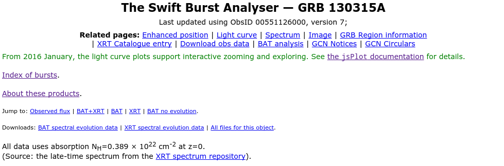
An example Data Overview section is below. This section contains some general information applicable to all of the data on the page, and some useful links. Below the title of the burst the most recent ObsID used in creating the plots is given, and the version of that ObsID. This can be compared to the Quick-look site to determine whether the page has been automatically updated with the most recent data delivery yet. After links to a few related pages and links to the individual light-curve section are given links to a few useful files: BAT/XRT spectral evolution data, and a tar archive containing all of the files for this GRB.
The BAT and XRT spectral evolution data files are ASCII files (formatted for use with QDP) giving the hardness ratio light curve of the GRB in BAT or XRT, and this hardness ratio expressed as a counts-to-flux conversion factor or Photon index. The files contain 21 columns: seven properties each with a value, positive error and negative error. These properties are (in order): time, hardness ratio, 0.3—10 keV flux conversion factor, 15—50 keV flux conversion factor, photon index (Γ), flux density at 10 keV conversion factor and the native-band observed flux density conversion factor. The All files for this object link supplies a tar archive containing all burst analyser files for this object.
Following these links there may appear a warning if the BAT spectrum required a cut-off power law (see caveats for details). Then the absorption model used in the flux calculations is also given, and where it was determined from.
[Back to Results Pages | Back to top | Index of bursts]
For most GRBs there will be five light-curve sections: the observed flux in all available instruments; then the unabsorbed flux plots. These consist of the BAT and XRT data combined, then plots with each instrument separately. For BAT this latter plot includes times before the trigger and the time axis defaults linear scaling. The final plot is the BAT flux light curve without spectral evolution. For bursts without data from the BAT or XRT, only the relevant single-instrument plot(s) will be shown.
The light curve section begins with two links. Reliability checks summarises the sanity checks users should apply to the light curves. Show hardness ratio opens a new panel showing the measured hardness ratio of the GRB [for BAT this is the (25—50 keV)/(15—25 keV) ratio; for XRT (1.5—10 keV)/(0.3-1.5 keV)]. The hardness ratio can be shown either as the measured hardness ratio, or as the hardness ratio translated into spectral photon index or counts-to-flux conversion factor (see creation algorithm).
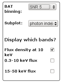
For the unabsorbed flux curves, the links are followed by up to three light curves: by default only the flux density at 10 keV is shown, however the options panel allows users to also show the 0.3—10 keV and 15—50 keV light curves. For the observed flux curve, only a single plot exists (each dataset in its own native energy band). Each light curve is preceded by some controls to manipulate the plot, and contains an options panel to the right of the plot to select which data are shown. These are discussed momentarily. For the observed flux plot, if UVOT data are present in the plot then a key explaining the colours is also shown.
Below the plots are links to generate a postscript version of the current plot and download the raw data.
Note: The on-screen plots are generated dynamically in javascript using
library developed at the UKSSDC, called jsplot.
At present, this cannot natively produce
postscript files, so instead it uses QDP/PGPLOT to make the postscript file.
jsplot was deliberately designed to behave like PGPLOT
so that the postscript files are as similar as possible to the on-screen plot, however
subtle differences are possible.
The plots can be easily rescaled using the mouse. Left-click and drag to select a region, and the plot will automatically zoom in to that part of the plot. If the plot had multiple panels (e.g. flux at the top and photon index below) the time axes of the two plots are tied. To return to the original scaling, press escape, or click on the “Restore” button which appears above the plot. You can also zoom in and out using the mouse scroll wheel (or equivalent on a touch pad), if you hold the control or shift keys. Control+scroll will cause the window to zoom in or out keeping the axis centres unchanged. Using shift+scroll will zoom in or out centred about the mouse location. To toggle whether the axes are linear or logarithmic, use the check boxes above the plot. Note that if you have linear axes which extend to (or below) zero, and then select log axes, you will get an error. Other controls are described in the jsplot documentation.
For more fine control, or for users who cannot/do not wish to use the mouse to zoom (e.g. on touchscreen devices, which jsplot does not currently support) a link is provided above the plot, entitled, “Show full <plot type> plot controls.” This will then display a form where the limits of each axis can be set; click “Plot” to replot the data.
The burst analyser light curves can be customised to some extent, in addition to the rescaling of the axes described above. To the right of the first plot in each section is a box with various controls. The controls are detailed below — note that not all controls are available for each light curve.
[Back to Results Pages | Back to top | Index of bursts]
For full details of how the burst analyser unabsorbed flux curves are created, users are directed to Evans et al. (2010, A&A, 519, 102). A summary is given here, along with details of how the observed flux density curves and UVOT data are produced. The process of creating the fluxed light curves can be split into three phases: building the count-rate light curves and hardness ratios; determining the conversion factors; creating the fluxed light curves.
The XRT count-rate light curves and hardness ratios are taken directly from the XRT light curve repository. See Evans et al. (2007, 2009) for details. The hardness ratio is rebinned to contain at least 20 photons per band, per bin. This helps to avoid low significance fluctuations in hardness from creating artificial features in the light curves.
For BAT, first the batbinevt tool, with the detector mask and total event list
produced by batgrbproduct. Signal-to-noise (SNR) binned light curves are then built from
this 40-ms light curve for SNR 4,5,6 and 7 using a custom script which bins the
highest-significance bins first so as to maximise both SNR and time resolution. No bin is allowed
to exceed 40 s in duration. If a bin reaches 40 s and is still not at the SNR threshold, it will
be written regardless. If it has SNR<2 it will be preceeded with an !. This means that, while
the bin is still present in the data file which can be viewed and downloaded, it is not shown in
the online plots (unless specifically requested). A second set of SNR-binned light curves are created where only data from T>0
are included. We create the second set for use with the XRT and UVOT data (which is plotted in
log-log space and so cannot include times at or before the trigger) because this ensures that the binning
is optimised for the data which are displayed, which would not be true if we simply ignore the bins at T<0
from the full light curve.
In addition to the SNR-binned light curves, 15—150 keV light curves with fixed-duration bins
are created using batbinevt, for bin sizes of 4 ms, 64 ms, 1 s and 10 s†. These light curves do not cover the
entire event list (since this would produce many bins composed entirely of noise), but the time range given by:
T90,start−1.05T90 ≤ t ≤ T90,end+1.05T90
where T90,start and T90,end
mark the time region over which T90 was accumulated, according to batgrbproduct.
A hardness ratio time series is created in a similar manner to the SNR-binned light curves. 15—25 keV
and 25—50 keV 4-ms binned light curves are created from the total BAT event list using
batbinevt. These are then passed to the SNR-binning code which requires SNR≥5 in
each band in order to create a bin (the maximum bin size is again 40 s.) If fewer than 3 bins with
SNR≥3 were created the target SNR is reduced to 4 and the hardness ratio is rebuilt; and again
with a target SNR of 3 if necessary. Even if this does not produce more than 2 "good"
bins the SNR is not further reduced.
† Not all of these bin durations are used for every GRB. Bin durations which are longer than T90 are not created. Similarly a 4-ms binned light curve is not created if T90 is longer than 10 s.
[Back to Creation Algorithm | Back to top | Index of bursts]
In an ideal world, to track spectral evolution and thus create a time-dependent counts-to-flux
conversion factor, one would create and fit a spectrum for each light curve bin. In reality this
is impossible since there are insufficient photons per bin to create a usable spectrum. Instead we
assume a spectral shape and use the hardness ratio to track the evolution of that spectrum. The
spectral shape used is either a power-law or a cut-off power-law. The choice of which to use is
made by fitting the BAT T90 spectrum (from batgrbproduct). If the cut-off
power-law model improved χ2 by at least 9 (a 3-σ improvement) the cut-off
power law is used (for BAT and XRT), otherwise a power-law is adopted. Note that, using a single hardness ratio we
cannot track the evolution of both power-law index and cut-off energy, therefore if a cut-off
model is required the cut-off energy is frozen at the value obtained from the fit to the
T90 spectrum. See caveat 2 for more details.
As well as a spectral shape, an absorption model is needed‡. If there are
XRT data for the GRB the absorption is taken from this. As Butler
& Kocevski (2007) demonstrated that absorption measures
calculated from early-time XRT spectra can be incorrect, if there are
at least 200 X-ray photons detected at t>4000 s, an X-ray spectrum
is constructed from data after this time, and the absorption is
determined from an absorbed power-law model which is automatically
fitted to this spectrum. Otherwise the absorption from the spectrum on
the XRT spectrum
repository is used. This absorption is made of two components, a
Galactic absorber and an intrinsic absorber. If the redshift of the
GRB is known, the intrinsic component is given this redshift. If no
XRT data exist for the burst, the Galactic column at the BAT position
is obtained from the nhtot tool
created by Willingale et al. (2013),
and the intrinsic component is given NH=1022 cm-2 at z=2.3; these are typical values for XRT spectra
(see Evans
et al. 2009). The absorption model used, and whence it was
determined, is shown on the results web
pages immediately before the light curve plots begin.
The power-law or cut-off power-law spectral model, absorption and instrumental response
matrices are then loaded into xspec and the
photon index (Γ) is stepped from -1 to +5 in steps of 0.1 (note:
N(E)∝E-Γ) For each Γ value, the hardness ratio, count-rate, flux
(0.3—10 keV and 15—50 keV) and flux density§
(both absorbed and observed) are calculated. This yields a lookup table which translates hardness ratio to Γ and to
counts-to-flux(-density) conversion factor. Using this table each point in the hardness ratio is
then converted into Γ and the necessary conversion factors, by interpolating this lookup
table. For BAT data there may be some times where the hardness ratio was negative (when the burst
is faint and no SNR≥3 hardness bin could be made). These cannot be converted to conversion
factors, so are skipped.
For the non-spectrally evolving BAT fluxed light curve the process is much simpler. The
best-fitting T90 spectrum is loaded into xspec and the count-rate, fluxes
and flux density are calculated. These give the time-averaged counts-to-flux(-density) conversion
factors. Note that no XRT non-spectrally evolving light curve is created as part of this project
since this is already supplied by the XRT light curve
repository.
‡ The light curves are all given as intrinsic, i.e. unabsorbed, flux (or flux density).
§ The normalisation parameter of the power-law and
cut-off power-law models in xspec is defined as the flux
density at 1 keV, in units of photons keV-1 cm-2
s-1, which is thus converted to Jy by multiplying by
0.000662, and can be extrapolated to the flux density at 10 keV
because the spectral model is known.
[Back to Creation Algorithm | Back to top | Index of bursts]
The final stage involves taking each bin in the count-rate light curves, interpolating the "hardness-ratio-as-conversion-factors" data produced in the previous step to determine the conversion factor at the centre of the bin, and then multiplying the count-rate by this value. The uncertainty in the conversion factor is not propagated into the final flux error bar (discussed below). Where there are gaps in the BAT "hardness-ratio-as-conversion-factors" data due to negative hardness ratios the conversion factor is interpolated across this gap. Due to the significant spectral evolution seen during the prompt emission of a GRB, we do not extrapolate the BAT "hardness-ratio-as-conversion-factors" to times before (after) the first (last) bins with a positive hardness ratio. However for XRT, because of the way the XRT light curves are created it is only ever the final bins which may not have corresponding hardness ratio information. Since XRT data do not generally show spectral evolution after the first few hundred seconds, the final measured hardness ratio value (and hence conversion factors) is applied to all light curve bins which occur after the hardness ratio finishes.
[Back to Creation Algorithm | Back to top | Index of bursts]
The UVOT light curves are not generated at the UKSSDC, but instead taken
from the Swift ground analysis web pages.
Data are uploaded here by the UVOT team only after manual checks for obvious problems
(such as source confusion, or poor aspect solutions) have been performed.
If UVOT data for the burst are available on this site, the FITS file is downloaded,
and the flux density information is extracted from this (the FLUX_HZ column, and
associated errors), along with the limiting flux for the exposure: this is a 2-σ limit. For each bin, if the
flux is above the limiting flux, the data point is saved as a detection, otherwise an upper limit
is saved.
If there are at least 2 detections in different filters, the UVOT data can also be renormalised to a single band, to make the overall behaviour of the UV/optical light curve easier to see. Note that this implicitly assumes all UVOT filters evolve in step with no spectral evoltuion. To renormalise, a fit is performed simultaneously to the UVOT detections from all filters. The model fitted is a (broken) power-law, with the same decay index for all filters but the normalisation for each filter able to vary independently. Fits with 0—3 breaks are attempted, a break only being accepted if it represents at least a 3-σ improvement over the previous best fit, according to an f-test (i.e. the probability of a chance improvement of χ2 is less than 0.3%). When the best-fitting model is determined, all data points and upper limits for the filters included in the fits are renormalised to a common band, using the best-fitting normalisations. Filters with only upper limits cannot be renormalised.
Ideally all UVOT GRB light curves would be renormalised to the same filter, but this is not possible since there is no filter in which all UVOT-detected GRBs were detected. Therefore, the filter to which the data are renormalised is chosen from the following list. The first entry in this list in which the GRB was detected is that to which the data are normalised.
Caution should be used when interpreting the renormalised UVOT data, as explained in the UVOT caveats section, below.
[Back to Creation Algorithm | Back to top | Index of bursts]
Although every effort has been made to ensure the reliability of these light curves, blind usage is not recommended. Users are strongly encouraged to read this section, and to ask the five reliability questions about every burst.
As discussed in the algorithm section above, the uncertainty in counts-to-flux error is not propagated into the final fluxed light curve. This is because the effect is at least partially systematic and propagating this uncertainty has the effect of 'washing out' genuine light curve features. However, it is important to check the uncertainty in the conversion factor, especially where surprising results are seen. If the Conversion Factor or Γ subplots show large errors (see products pages for how to view these) the final flux value is also much less precise than suggested by its error bar.
Related to the above caveat: because negative hardness ratios are impossible in reality (they arise in the data due to Poisson noise) when converting the hardness ratio to Γ and counts-to-flux conversion factor the negative error on the hardness ratio is necessarily truncated to give HRmin=0. This means that the negative errors on Γ and the conversion factor are also truncated and thus unreliable. This can usually be readily determined by eye because the errors on these properties are highly asymmetric. Alternatively, users can check the hardness ratio: if the minimum value is zero, the uncertainty in Γ/conversion factor has been truncated.
As noted earlier, while the facility exists to hide the UVOT upper limits, this should only be used for cosmetic purposes, to allow you to identify where the detection exist. Ignoring non-detections in any analysis will bias your conclusions.
While the BAT and XRT data have been converted from counts to flux using time-dependent
spectral information to track spectral evolution, all UVOT flux units are generated
using the assumption of a single fixed GRB spectrum, as described
in the uvotsource help.
Similarly, when renormalising the UVOT data to a common band, it has to be implicitly assumed that the
filters are evolving in step, that is, none of the sychrotron break frequencies pass through the UVOT band
(or they pass through very rapidly). These assumptions may not be reliable:
Oates et al. (2012) showed
that the spectral index of GRBs varies significantly from burst to burst, and
Schady et al. (2010) showed
that the extinction (for which the UVOT light curves are not corrected) also shows
significant variation. Therefore, while the UVOT data can be used to track the decay rate of the GRB
in the optical and UV bands, to create an SED from these data requires in depth and careful analysis.
Source confusion can also occasionally be an issue for UVOT data. While UVOT light curves should not be uploaded to GCN (and therefore picked up by the burst analyser) without manually checking for this, this checking is not 100% reliable. Users can check for source confusion themselves by obtaining the UVOT data from the archive and comparing the image near the GRB with a catalogue image (e.g. DSS) and verifying that the afterglow is not present in the catalogue.
In order to convert the count-rate light curves into flux we need some spectral information. As described above we do this using hardness ratios as we do not have enough data to create accurate spectra for each light curve bin. However, this approach implicitly assumes a spectral shape (either a power-law or cut-off power law). For the light curves where the flux is given within the band pass of the instrument (i.e. the BAT 15-50 keV and XRT 0.3-10 keV light curves), this assumption is usually supportable; however when extrapolating the flux outside the observed band, if the spectral shape is not that assumed, the results may be incorrect. This is why the default light curve on the web pages is the flux density at 10 keV; this value allows us to directly compare BAT and XRT data, but minimises the extrapolation.
The five questions below can be used to identify cases where the fluxed light curves may be unreliable. More details, and what to do in each case, follow the list.
A fundamental assumption used to create the fluxed light curves is that the spectral slope is the same in the BAT (15-50 keV) and XRT (0.3-10 keV) bandpasses at a given time. If this is not true, the extrapolated fluxes may be inaccurate. For example, consider the case where the true spectral shape is a broken power-law with a break between the XRT and BAT bands, and a steeper index above the break. The BAT count-rate will be converted to 0.3-10 keV flux using an erroneously soft spectrum and will thus overestimate the flux. Similarly the XRT count-rate will be converted to 15-50 keV count-rate using a spectral index which is too hard and again will overestimate the flux.

This circumstance is readily identified by looking at the Γ values which accompany the light curves. In the example to the right, GRB 060526, the BAT Γ values at 200-400 s are systematically higher (softer) than the XRT values. The 0.3-10 keV light curve and 15-50 keV light curve show the effects discussed above. However as the break must lie somewhere between the bands, the effect of this inaccuracy on the flux density at 10 keV is minimal and indeed the BAT and XRT flux value here agree well.
In summary: If the Γ values are discontinuous between BAT and XRT the flux value outside of the instruments' bandpasses are unreliable. The flux density at 10 keV is the most immune to this problem.
[Back to the 5 questions | Back to top | Index of bursts]
The BAT spectrum cannot always be adequately described as a power-law. In the event that a cut-off power-law (CPL) fit improves χ2 by at least 9 (i.e. the CPL fit offers a 3-σ improvement over the power-law fit) this model will be used to generate the counts-to-flux conversion factors (for both BAT and XRT). However, to track the evolution of both the photon index and the cut-off energy is not possible; this requires two hardness ratios and there is usually insufficient signal-to-noise to generate such data. Further, if the cut-off energy is towards the edge or outside of the bandpass covered by BAT or XRT a strong degeneracy between this energy and the photon index arises. Consequently, when a CPL model is required by the BAT spectrum, the cut-off energy is frozen at the value determined from the T90 spectrum. In reality we expect the cut-off energy to be evolving with time, thus fixing the parameter introduces an extra source of uncertainty in the counts-to-flux conversion which is not reflected in the errors. As with discontinuous Γ values, this effect is likely to be strongest when considering the flux extrapolated outside of the instruments' own bandpasses. Although experience shows that the effect of this is minimal, users should be aware of this, and be cautious ascribing weight to outlying data points where a CPL spectrum has been used. If a CPL spectrum was used, this is reported prominently on the results page, with a sentence such as the following given before any of the light curves:
The BAT spectrum was fitted with a cut-off power-law. The cutoff energy was 93.9 keV and was not allowed to evolve. See caveats for details.
In summary: If a cut-off power-law spectral fit was required by BAT, the uncertainty in counts-to-flux conversion may be underestimated, especially when extrapolating outside the instruments' bandpasses.
[Back to the 5 questions | Back to top | Index of bursts]
As described above, the Γ values given for each light-curve bin are not determined from spectral fits, but from the hardness ratio. Extreme values (outside the range ~0-4) are not generally seen in fitted spectra (see The Swift Data Table and The XRT catalogue paper) and thus may indicate low signal hardness ratios. These should be accompanied by large error bars, and the associated warnings should be taken into account. Note further that the look-up table from hardness ratio to Γ/conversion factor is only determined for -1 ≤ Γ ≤ 5. Thus Γ values outside this range have been extrapolated beyond the range over which the relationship is calibrated. Again, this should be reflected in large uncertainties in Γ. In general, where the Γ values are outside the 0—4 range (and certainly outside the -1—5 range) the flux points should be viewed with caution.
In summary: Any flux points with corresponding Γ values outside the range 0 ≤ Γ ≤ 4 should be viewed with caution.
[Back to the 5 questions | Back to top | Index of bursts]
This topic is discussed in detail in the discussion of error bars.
By default, BAT points with 'bad' conversion factors are not shown in the online plots. A 'bad' conversion factor is defined as either being consistent with zero, or having an error larger than two orders of magnitude (positive or negative). Such points are still present in the data file; these points are indicated by a !# at the start of the line. Selecting the Show 'bad' points option causes these data points to be included in the plot.
In summary: Errors on Γ and conversion factor have not been propagated to the flux light curves. Where the hardness ratio is consistent with 0 the negative error on Γ and conversion factors are underestimates.
[Back to the 5 questions | Back to top | Index of bursts]
Spectral evolution is accounted for by tracking the hardness ratio evolution, interpolating between measured values to the times of light-curve bins. In fainter bursts there may be only one or two hardness ratio bins. In such cases we cannot track the evolution and the spectrum will tend towards the non-evolving flux spectrum. This can be seen from the Γ or conversion factor sub-plots, since a single hardness ratio point will result in each bin in the sub-plot being the same. This does not give an inaccuracy in the fluxed light curve (provided the errors on the conversion factor are considered), but it does mean that the effects of spectral evolution are not visible in the light curve but rather hidden in the uncertainty in the conversion factor.
In summary: If the Γ or conversion factors are not varying there was minimal hardness ratio information, so the effects of spectral evolution are not visible in the fluxed light curve.
[Back to the 5 questions | Back to top | Index of bursts]
[Back to top | Index of bursts]
As with all automated products supplied by the UKSSDC, these light curves are built and updated as soon as data become
available◊. Since
BAT and XRT data do not necessarily arrive at the same time, the BAT and XRT portions of the Burst
Analyser products can be built independently. This may mean that initially for a newly-detected
burst there may be only a BAT or XRT light curve. The building of the BAT products occurs when the
BAT data first arrive, or the ONTIME of the BAT data on the quick-look site increases compared to that
available when the light curves were last built. For the XRT data, when the light curve repository builds or updates the
count-rate light curve it sets a flag which causes the Burst Analyser to build or update the flux
light curve.
◊ Building or updating of light curves is triggered by a cron job which
runs every ten minutes.
[Back to top | Index of bursts]
There are no restrictions on the use of these products, however we do request acknowledgement. Where data from the Burst Analyser are used, please cite the paper Evans et al. (2010, A&A, 519, 102). If you use the count-rate light curves to which the Burst Analyser provides links, please note they they also require acknowledgement: for BAT data please acknowledge Taka Sakamoto and Scott D. Barthelmy, for XRT data please cite Evans et al. (2009, MNRAS, 397, 1177) and Evans et al. (2007, A&A, 469, 379).
Also, wherever these data are used please include the following text in the acknowledgements: This work made use of data supplied by the UK Swift Science Data Centre at the University of Leicester.
[Back to top | Index of bursts]
Any changes made to the software after the paper is published are shown here.
[Back to top | Index of bursts]
UK Swift Science Data Centre
Last updated 2011 June 07 at 13:26 UT
Web page maintained by Phil Evans
E-mail: swift help
Please read our privacy notice.